Linear Discriminant Analysis and Logistic Regression Matthieu R. - PDF document

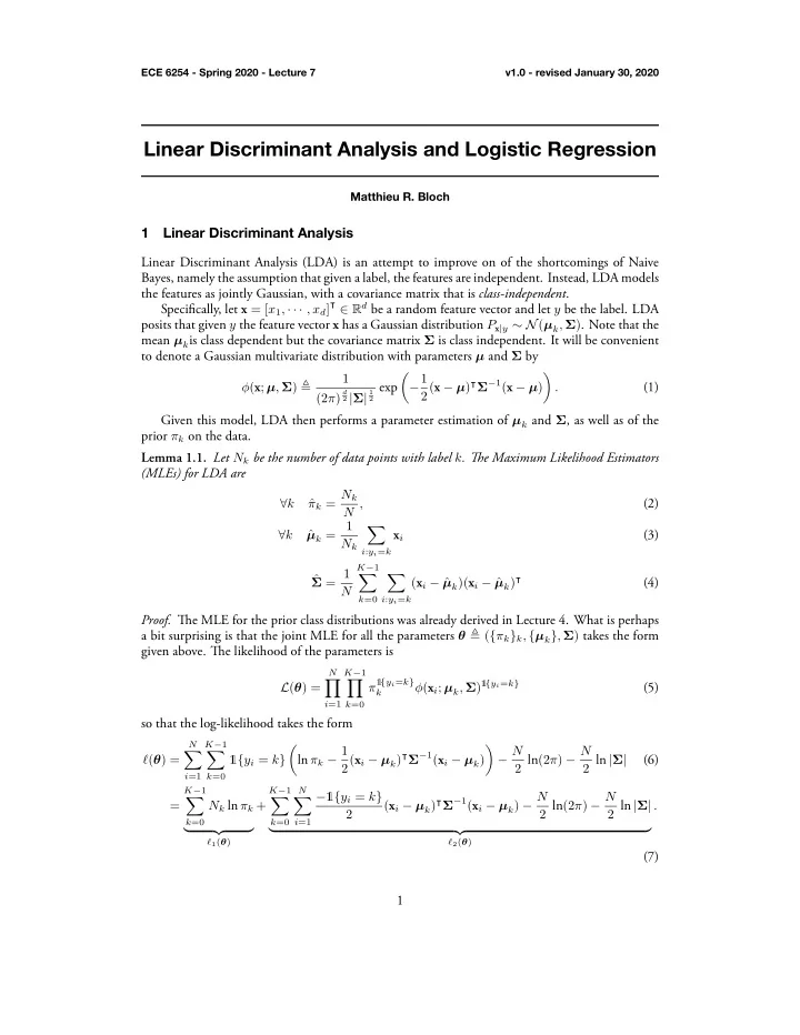
1 (1) (7) (6) so that the log-likelihood takes the form (5) Linear Discriminant Analysis (LDA) is an attempt to improve on of the shortcomings of Naive Bayes, namely the assumption that given a label, the features are independent. Instead, LDA models the features as jointly Gaussian, with a covariance matrix that is class-independent . given above. Tie likelihood of the parameters is Proof. Tie MLE for the prior class distributions was already derived in Lecture 4. What is perhaps (4) (3) (2) (MLEs) for LDA are ECE 6254 - Spring 2020 - Lecture 7 v1.0 - revised January 30, 2020 Linear Discriminant Analysis and Logistic Regression Matthieu R. Bloch 1 Linear Discriminant Analysis Specifically, let x = [ x 1 , · · · , x d ] ⊺ ∈ R d be a random feature vector and let y be the label. LDA posits that given y the feature vector x has a Gaussian distribution P x | y ∼ N ( µ k , Σ ) . Note that the mean µ k is class dependent but the covariance matrix Σ is class independent. It will be convenient to denote a Gaussian multivariate distribution with parameters µ and Σ by � � 1 − 1 2( x − µ ) ⊺ Σ − 1 ( x − µ ) ϕ ( x ; µ , Σ ) ≜ . d 1 2 | Σ | 2 exp (2 π ) Given this model, LDA then performs a parameter estimation of µ k and Σ , as well as of the prior π k on the data. Lemma 1.1. Let N k be the number of data points with label k . Tie Maximum Likelihood Estimators π k = N k ∀ k ˆ N , µ k = 1 � ∀ k ˆ x i N k i : y i = k K − 1 Σ = 1 � � ˆ µ k ) ⊺ ( x i − ˆ µ k )( x i − ˆ N k =0 i : y i = k a bit surprising is that the joint MLE for all the parameters θ ≜ ( { π k } k , { µ k } , Σ ) takes the form K − 1 N � � { y i = k } π 1 ϕ ( x i ; µ k , Σ ) 1 { y i = k } L ( θ ) = k i =1 k =0 K − 1 N � � ln π k − 1 − N 2 ln (2 π ) − N � � 2( x i − µ k ) ⊺ Σ − 1 ( x i − µ k ) 1 { y i = k } 2 ln | Σ | ℓ ( θ ) = i =1 k =0 K − 1 K − 1 N − 1 { y i = k } ( x i − µ k ) ⊺ Σ − 1 ( x i − µ k ) − N 2 ln (2 π ) − N � � � 2 ln | Σ | = N k ln π k + . 2 k =0 k =0 i =1 � �� � � �� � ℓ 1 ( θ ) ℓ 2 ( θ )

2 (8) Proof. Tie first part of the lemma follows by remembering that for a plug-in classifier, we have (14) Lemma 1.2. Tie LDA classifier is this again in the context of bias-variance tradeoff. points gets large. In practice, you could choose any other estimator of your liking, we will discuss yields You might notice that the covariance estimator is biased , but the bias vanishes as the number of (13) we obtain (check the matrix cookbook for the derivation rules) (12) (11) tr (10) (9) ECE 6254 - Spring 2020 - Lecture 7 v1.0 - revised January 30, 2020 Note that { π k } do not interact with { µ k } and Σ . Consequently, the MLE of { π } k is the one we N where N k = � N studied previously and π k = N k i =1 1 { y i = k } . Let us focus on maximizing ℓ 2 ( θ ) . Taking the gradient with respect to µ k and setting it to 0 K − 1 N ∂ℓ 2 ( θ ) − 1 { y i = k } � � � � − 2 Σ − 1 x i + 2 Σ − 1 µ k = ∂ µ k 2 k =0 i =1    � = Σ − 1 x i − N k µ k  x i : y i = k = 0 Conveniently, note that Σ − 1 (assumed non-singular) does not enter the equation and we obtain � 1 µ k = x i : y i = k x i . N k Finally, to take the gradient with respect to Σ , we rewrite ℓ 2 ( θ ) as K − 1 N − 1 { y i = k } − N 2 ln (2 π ) − N � � � � ( x i − µ k ) ⊺ Σ − 1 ( x i − µ k ) ℓ 2 ( θ ) = 2 ln | Σ | 2 i =1 k =0     K − 1   = − 1 − N 2 ln (2 π ) − N � � ( x i − µ k )( x i − µ k ) ⊺  Σ − 1  2 ln | Σ |   2 tr   k =0 x i : y i = k   � �� � ≜ S ∂ℓ 2 ( θ ) = − 1 = 1 − Σ − 1 S Σ − 1 − N Σ − 1 � 2 Σ − 1 ( S Σ − 1 − N I ) = 0 � ∂ Σ 2 Again, for Σ − 1 non singular, we obtain Σ = S ■ N . � 1 � µ k ) ⊺ ˆ − 1 ( x − ˆ 2( x − ˆ µ k ) − log ˆ h LDA ( x ) = argmin Σ π k k For K = 2 , the LDA classifier is a linear classifier.

3 (17) (23) argmax LDA. You should check for yourself that With Vapnik’s word of caution in mind, let us revisit one last time the binary classifier with LDA is, in Vapnik’s words, that ” one should solve the [classification] problem directly and never solve An natural extension of LDA is Quadratic Discriminant Analysis (QDA), in which we allow (15) without other tricks (dimensionality reduction, structured covariance) that we will discuss later. test in (22) is simply checking on what side of the hyperplane the point x lies. (22) (21) (19) (16) (18) ECE 6254 - Spring 2020 - Lecture 7 v1.0 - revised January 30, 2020 h ( x ) ≜ argmax k η k ( x ) . Here, η k ( x ) = argmax P y | x ( k | x ) k k ( a ) = argmax P x | y ( x | k )ˆ π k k ( b ) � log P x | y + log ˆ � = argmax π k k � � 2 � � � � 1 − 1 µ k ) ⊺ ˆ − 1 ( x − ˆ d � ˆ � � − log 2( x − ˆ = argmax (2 π ) Σ Σ µ k ) + log ˆ π k 2 � k � 1 � ( c ) µ k ) ⊺ ˆ − 1 ( x − ˆ = argmin 2( x − ˆ µ k ) − log ˆ Σ π k , k where ( a ) follows by Bayes’ rule and the fact that P x does not depend on k ; ( b ) follows because x �→ log x is increasing; ( c ) follows by dropping all the terms that do not depend on k and the fact that argmax x f ( x ) = argmin x − f ( x ) . For K = 2 , notice that the classifier is effectively performing the test η 0 ( x ) ≶ η 1 ( x ) ⇔ 1 π 0 ≷ 1 − 1 ( x − ˆ − 1 ( x − ˆ µ 0 ) ⊺ ˆ µ 1 ) ⊺ ˆ 2( x − ˆ Σ µ 0 ) − log ˆ 2( x − ˆ Σ µ 1 ) − log ˆ π 1 (20) − 1 x + 1 − 1 ˆ − 1 x + 1 − 1 ˆ µ ⊺ µ ⊺ µ ⊺ µ ⊺ 0 ˆ 0 ˆ 1 ˆ 1 ˆ π 0 ≷ − ˆ ⇔ − ˆ Σ 2 ˆ Σ µ 0 − log ˆ Σ 2 ˆ Σ µ 1 − log ˆ π 1 x + 1 − 1 ˆ π 0 − 1 − 1 ˆ − 1 µ 0 ) ⊺ ˆ µ ⊺ µ ⊺ 0 ˆ 1 ˆ ≷ 0 ⇔ (ˆ µ 1 − ˆ Σ 2 ˆ Σ µ 0 − log ˆ 2 ˆ Σ µ 1 + log ˆ π 1 � �� � � �� � ≜ w ≜ b ⇔ w ⊺ x + b ≷ 0 . Tie set H ≜ { x ∈ R d : w ⊺ x + b = 0 } is a hyperplane , which is an affine subspace of R d of dimension d − 1 . H acts as a linear boundary between the two classes that we are trying to distinguish, and the ■ To conclude on LDA, note that the generative model P x | y ∼ N ( µ , Σ ) is rarely accurate. In addition, there are quite a few parameters to estimate, including K − 1 class priors, Kd means, 1 2 d ( d + 1) elements of covariance matrix. Tiis works well if N ≫ d but works poorly if N ≪ d the covariance matrix Σ k to vary with each class k . Tiis results in a quadratic decision boundary instead of the linear boundary established in Lemma 1.2. However, perhaps the biggest issue with a more general problem as an intermediate step [such as modeling P ( x | y ) ]. ”. With LDA, as should be clear from Lemma 1.1, we are actually modeling the entire joint distribution P x ,y , when we really only care about η k ( x ) for classification. µ 1 , ˆ π 1 ϕ ( x ; ˆ ˆ Σ ) 1 η 1 ( x ) = = 1 + exp ( − ( w ⊺ x + b )) , µ 1 , ˆ µ 0 , ˆ ˆ π 1 ϕ ( x ; ˆ Σ ) + ˆ π 0 ϕ ( x ; ˆ Σ )

4 (24) (27) parameters (see (22)) to compute these parameters as a function of the mean and covariance matrix of a Gaussian distri- bution. Tie direct estimation of these parameters leads to another linear classifier called the logistic classifier . Tiis is again a linear classifier. Note that LDA led to a similar classifier with the specific choice of (26) name and is defined as (25) ECE 6254 - Spring 2020 - Lecture 7 v1.0 - revised January 30, 2020 where w and b are defined as per (22). In other words, we do not need to estimate the full joint distribution. All that seems to be required are the parameters w and b , and LDA makes a detour 2 Logistic regression Tie key idea behind (binary) logistic regression is to assume that η 1 ( x ) is of the form 1 1 + exp ( − ( w ⊺ x + b )) ≜ 1 − η 0 ( x ) , w and ˆ and to directly estimate ˆ b from the data. One therefore obtains an estimate of the conditional distribution P y | x (1 | x ) as 1 η 1 ( x ) = . w ⊺ x + ˆ 1 + exp ( − (ˆ b )) 1 Since the function x �→ 1+ e − x is called the logistic map , the corresponding classifier inherited the � � η 1 ( x ) ⩾ 1 � � w ⊺ x + ˆ b ⩾ 0 h LR ( x ) = 1 = 1 ˆ . 2 b = 1 − 1 ˆ µ 0 − 1 − 1 ˆ µ 1 + log ˆ π 1 − 1 (ˆ µ ⊺ µ ⊺ w = ˆ 0 ˆ 1 ˆ ˆ µ 1 − ˆ µ 0 ) 2 ˆ 2 ˆ Σ Σ Σ ˆ π 0 Note that this not what the MLE of (ˆ w , b ) would result in, and we will analyze this in more details.