Day 3: Classification Lucas Leemann Essex Summer School - PowerPoint PPT Presentation
Day 3: Classification Lucas Leemann Essex Summer School Introduction to Statistical Learning L. Leemann (Essex Summer School) Day 3 Introduction to SL 1 / 33 1 Motivation for Classification 2 Logistic Regression The Linear
�� Day 3: Classification Lucas Leemann Essex Summer School Introduction to Statistical Learning L. Leemann (Essex Summer School) Day 3 Introduction to SL 1 / 33
�� 1 Motivation for Classification 2 Logistic Regression The Linear Probability Model Building a Model from Probability Theory 3 Linear Discriminant Analysis Building a Model from Probability Theory Example 1 (k=2) Example 2 4 Comparison of Classification Methods L. Leemann (Essex Summer School) Day 3 Introduction to SL 2 / 33
�� Classification Standard data science problem, i.e. • who will default on credit loan? • which customers will come back? • which e-mails are spam? • which ballot stations manipulated the vote returns? • who is likely to vote for which party? L. Leemann (Essex Summer School) Day 3 Introduction to SL 3 / 33
�� Logistic Regression L. Leemann (Essex Summer School) Day 3 Introduction to SL 4 / 33
�� Linear Probability Model LPM The linear probability model relies on linear regression to analyze binary variables. Y i = β 0 + β 1 · X 1 i + β 2 · X 2 i + ... + β k · X ki + ε i Pr ( Y i = 1 | X 1 , X 2 , ... ) = β 0 + β 1 · X 1 i + β 2 · X 2 i + ... + β k · X ki Advantages: • We can use a well-known model for a new class of phenomena • Easy to interpret the marginal e ff ects of X L. Leemann (Essex Summer School) Day 3 Introduction to SL 5 / 33
�� Problems with Linear Probability Model The linear model needs a continuous dependent variable, if the dependent variable is binary we run into problems: • Predictions, ˆ y , are interpreted as probability for y = 1 → P ( y = 1) = ˆ y = β 0 + β 1 X , can be above 1 if X is large enough → P ( y = 0) = ˆ y = β 0 + β 1 X , can be below 0 if X is small enough • The errors will not have a constant variance. → For a given X the residual can be either (1- β 0 - β 1 X ) or ( β 0 + β 1 X ) • The linear function might be wrong → Imagine you buy a car. Having an additional 1000 £ has a very di ff erent e ff ect if you are broke or if you already have another 12,000 £ for a car. L. Leemann (Essex Summer School) Day 3 Introduction to SL 6 / 33
�� Predictions can lay outside I = [0 , 1] Binary Dependent Variable 1.0 0.8 Actual Values 0.6 Prediction >100% 0.4 0.2 0.0 0.0 0.5 1.0 1.5 2.0 Predicted Values Residuals if the dependent variable is binary: Continuous Dependent Variable Binary Dependent Variable 6 0.8 Predicted Values Predicted Values 5 0.6 4 3 0.4 2 1 0.2 -5 0 5 10 15 20 -0.5 0.0 0.5 Residuals Residuals L. Leemann (Essex Summer School) Day 3 Introduction to SL 7 / 33
�� Predictions should only be within I = [0 , 1] • We want to make predictions in terms of probability • We can have a model like this: P ( y i = 1) = F( β 0 + β 1 X i ) where F( · ) should be a function which never returns values below 0 or above 1 • There are two possibilities for F( · ) : cumulative normal ( Φ ) or logistic ( ∆ ) distribution Cumulative Distribution 1.0 0.8 0.6 Y 0.4 Logistic Normal 0.2 0.0 -4 -2 0 2 4 β 0 + β 1 X L. Leemann (Essex Summer School) Day 3 Introduction to SL 8 / 33
�� Logit Model 1 The logit model is then: P ( y i = 1) = 1+exp( − β 0 − β 1 X i ) For β 0 = 0 and β 1 = 2 we get: 1.0 0.8 0.6 P(Y=1) 0.4 0.2 0.0 -2 -1 0 1 2 x L. Leemann (Essex Summer School) Day 3 Introduction to SL 9 / 33
�� Logit Model: Example 1.0 P(Y=1), `Taxes Are Too High' 0.8 0.6 0.4 0.2 0.0 20000 40000 60000 80000 100000 120000 Income in GBP 1 • We can make a prediction by calculating: P ( y = 1) = 1+exp( − β 0 − β 1 · X ) L. Leemann (Essex Summer School) Day 3 Introduction to SL 10 / 33
�� Logit Model: Example 1.0 P(Y=1), `Taxes Are Too High' P(y=1)=F(1-2*x) 0.8 P(y=1)=F(0-2*x) P(y=1)=F(1-1*x) 0.6 0.4 0.2 0.0 20000 40000 60000 80000 100000 120000 Income in GBP • A positive β 1 makes the s-curve increase. • A smaller β 0 shifts the s-curve to the right. • A negative β 1 makes the s-curve decrease. L. Leemann (Essex Summer School) Day 3 Introduction to SL 11 / 33
�� Example: Women in the 1980s and Labour Market > m1 <- glm(inlf ~ kids + age + educ, dat=data1, family=binomial(logit)) > summary(m1) Call: glm(formula = inlf ~ kids + educ + age, family = binomial(logit), data = data1) Deviance Residuals: Min 1Q Median 3Q Max -1.8731 -1.2325 0.8026 1.0564 1.5875 Coefficients: Estimate Std. Error z value Pr(>|z|) (Intercept) -0.11437 0.73459 -0.156 0.87628 kids -0.50349 0.19932 -2.526 0.01154 * educ 0.16902 0.03505 4.822 1.42e-06 *** age -0.03108 0.01137 -2.734 0.00626 ** --- Signif. codes: 0 *** 0.001 ** 0.01 * 0.05 . 0.1 1 (Dispersion parameter for binomial family taken to be 1) Null deviance: 1029.75 on 752 degrees of freedom Residual deviance: 993.53 on 749 degrees of freedom AIC: 1001.5 L. Leemann (Essex Summer School) Day 3 Introduction to SL 12 / 33
�� Example: Women 1980 (2) Call: glm(formula = inlf ~ kids + educ + age, family = binomial(logit), data = data1) Coefficients: Estimate Std. Error z value Pr(>|z|) (Intercept) -0.11437 0.73459 -0.156 0.87628 kids -0.50349 0.19932 -2.526 0.01154 * educ 0.16902 0.03505 4.822 1.42e-06 *** age -0.03108 0.01137 -2.734 0.00626 ** --- Signif. codes: 0 *** 0.001 ** 0.01 * 0.05 . 0.1 1 • Only interpret direction and significance of a coe ffi cient • The test statistic always follows a normal distribution ( z ) L. Leemann (Essex Summer School) Day 3 Introduction to SL 13 / 33
�� Example: Women 1980 (3) glm(formula = inlf ~ kids + educ + age, family = binomial(logit), data = data1) Coefficients: Estimate Std. Error z value Pr(>|z|) (Intercept) -0.11437 0.73459 -0.156 0.87628 kids -0.50349 0.19932 -2.526 0.01154 * educ 0.16902 0.03505 4.822 1.42e-06 *** age -0.03108 0.01137 -2.734 0.00626 ** • How can we generate a prediction for a woman with no kids, 13 years of education, who is 32? • Compute first the prediction on y ∗ , i.e. just compute β 0 + β 1 x 1 + β 2 x 2 + β 3 x 3 1 1 • P ( y = 1) = 1+ exp (0 . 11+ . 50 · 0 − 0 . 17 · 13+0 . 03 · 32) = 1+ exp ( − 1 . 09) = 0 . 75 L. Leemann (Essex Summer School) Day 3 Introduction to SL 14 / 33
�� Prediction > z.out1 <- zelig(inlf ~ kids + age + educ + exper + huseduc + huswage, model = "logit", data = data1) > average.woman <- setx(z.out1, kids=median(data1$kids), age=mean(data1$age), educ=mean(data1$educ), exper=mean(data1$exper), huseduc=mean(data1$huseduc), huswage=mean(data1$huswage)) > s.out <- sim(z.out1,x=average.woman) > summary(s.out) sim x : ----- ev mean sd 50% 2.5% 97.5% [1,] 0.5746569 0.02574396 0.5754419 0.5232728 0.6217502 pv 0 1 [1,] 0.432 0.568 L. Leemann (Essex Summer School) Day 3 Introduction to SL 15 / 33
�� Linear Discriminant Analysis L. Leemann (Essex Summer School) Day 3 Introduction to SL 16 / 33
�� Linear Discriminant Analysis • Why something new? • Might have more than 3 classes • problems of separation • Basic idea: We try to learn about Y by looking at the distribution of X • Logistic regression did this: Pr ( Y = k | X = x ) • LDA will exploit Bayes’ theorem and infer class probability directly from X and prior probabilities L. Leemann (Essex Summer School) Day 3 Introduction to SL 17 / 33
�� Basic Idea: Linear Discriminant Analysis (James et al, 2013: 140) L. Leemann (Essex Summer School) Day 3 Introduction to SL 18 / 33
�� Math-Stat Refresher: Bayes Doping tests: • 99% sensitive (correctly identifies doping abuse), P (+ | D ) = . 99 • 99% specific (correctly identifies appropriate behavior), P ( � | noD ) = . 99 • 0.5% athletes take illegal substances • You take a test and receive a positive result. What is the probability that you actually took an illegal substance? P ( D ) · P (+ | D ) P ( D | +) = P ( D ) · P (+ | D ) + P ( noD ) · P (+ | noD ) 0 . 005 · 0 . 99 P ( D | +) = 0 . 005 · 0 . 99 + 0 . 995 · 0 . 01 = 0 . 332 L. Leemann (Essex Summer School) Day 3 Introduction to SL 19 / 33
�� LDA: The Mechanics (with one X ) • We have X and it follows a distribution f ( x ) • We have k di ff erent classes • Based on Y , we can calculate the prior probabilities π k 1 Define f k ( x ) as the distribution of X for class k (p. 140/141) 2 Note: f k ( x ) = P ( X = x | Y = k ) 3 Hence: π k · f k ( x ) P ( Y = k | X = x ) = P K l =1 π l · f l ( x ) L. Leemann (Essex Summer School) Day 3 Introduction to SL 20 / 33
�� The Mechanics II P x i , k 1 f k ( x ) is assumed to be a normal distribution with µ k = and n k P K 1 i : y k = k ( x i � µ k ) 2 σ = P k =1 n − K σ 2 � µ 2 2 compute for each k : δ k ( x ) = x · µ k 2 σ 2 + log ( π k ) k 3 Classify i to be in k if δ k ( x ) > δ j ( x ) 8 j 6 = k L. Leemann (Essex Summer School) Day 3 Introduction to SL 21 / 33
�� Simple case: K=2 (James et al, 2013: 140) L. Leemann (Essex Summer School) Day 3 Introduction to SL 22 / 33
�� Example: Female Labor Force 80 60 not in labor force in labor force Frequency 40 20 0 0 10 20 30 40 Experience in years L. Leemann (Essex Summer School) Day 3 Introduction to SL 23 / 33
Recommend
More recommend
Explore More Topics
Stay informed with curated content and fresh updates.




![Classification Image Classification Set of predefined categories [eg: table, apple, dog, giraffe]](https://c.sambuz.com/743996/classification-s.webp)
