Systems Biology: Mathematics for Biologists Kirsten ten Tusscher, - PowerPoint PPT Presentation
Systems Biology: Mathematics for Biologists Kirsten ten Tusscher, Theoretical Biology, UU Chapter 4 Limit cycles N 0 20 0 2.5 5 R N t 5 10 10 15 20 0 2.5 5 R 15 5 0 R t 5 2.5 0 N 5 2.5 0 The classical
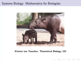
Systems Biology: Mathematics for Biologists Kirsten ten Tusscher, Theoretical Biology, UU
Chapter 4 Limit cycles
N 0 20 0 2.5 5 R N t 5 10 10 15 20 0 2.5 5 R 15 5 0 R t 5 2.5 0 N 5 2.5 0 The “classical” Lotka-Volterra model Consider the classical Lotka-Volterra predator-prey model. � d R d t = aR − bNR d N d t = cNR − dN with a = 1, b = 0 . 5, c = 0 . 25, d = 0 . 43. Note: no density-dependence, no saturation of predators.
N 0 20 0 2.5 5 R N t 5 10 10 15 20 0 2.5 5 R 15 5 0 R t 5 2.5 0 N 5 2.5 0 The “classical” Lotka-Volterra model Consider the classical Lotka-Volterra predator-prey model. � d R d t = aR − bNR d N d t = cNR − dN with a = 1, b = 0 . 5, c = 0 . 25, d = 0 . 43. Note: no density-dependence, no saturation of predators.
10 5 t N R 5 2.5 0 20 15 10 5 0 t 2.5 5 0 N 5 2.5 0 R 15 20 0 2.5 5 R N 0 The “classical” Lotka-Volterra model Consider the classical Lotka-Volterra predator-prey model. � d R d t = aR − bNR d N d t = cNR − dN with a = 1, b = 0 . 5, c = 0 . 25, d = 0 . 43. Note: no density-dependence, no saturation of predators. zero self-feedback due to horiz./vert. null-clines!
10 5 t N R 5 2.5 0 20 15 10 5 0 t 2.5 5 0 N 5 2.5 0 R 15 20 0 2.5 5 R N 0 The “classical” Lotka-Volterra model Consider the classical Lotka-Volterra predator-prey model. � d R d t = aR − bNR d N d t = cNR − dN with a = 1, b = 0 . 5, c = 0 . 25, d = 0 . 43. Note: no density-dependence, no saturation of predators. zero self-feedback due to horiz./vert. null-clines! neutrally stable equilibrium: center point
15 5 t N R 5 2.5 0 20 10 10 5 0 t 2.5 5 0 N 5 2.5 0 R 15 20 0 2.5 5 R N 0 The “classical” Lotka-Volterra model Consider the classical Lotka-Volterra predator-prey model. � d R d t = aR − bNR d N d t = cNR − dN with a = 1, b = 0 . 5, c = 0 . 25, d = 0 . 43. Note: no density-dependence, no saturation of predators. zero self-feedback due to horiz./vert. null-clines! neutrally stable equilibrium: center point initial conditions determine amplitude oscillations
Let us consider a more realistic LV-model First, we include density dependent growth of the prey:
Let us consider a more realistic LV-model First, we include density dependent growth of the prey: � d R d t = rR ( 1 − R K ) − bNR d N d t = cNR − dN
Let us consider a more realistic LV-model First, we include density dependent growth of the prey: � d R d t = rR ( 1 − R K ) − bNR d N d t = cNR − dN Second, we include a saturated functional response:
Let us consider a more realistic LV-model First, we include density dependent growth of the prey: � d R d t = rR ( 1 − R K ) − bNR d N d t = cNR − dN Second, we include a saturated functional response: d R d t = rR ( 1 − R � K ) − bNF R with F = d N d t = bNF − dN h + R
Let us consider a more realistic LV-model First, we include density dependent growth of the prey: � d R d t = rR ( 1 − R K ) − bNR d N d t = cNR − dN Second, we include a saturated functional response: d R d t = rR ( 1 − R � K ) − bNF R with F = d N d t = bNF − dN h + R R Substituting F = h + R this gives us: d R d t = rR ( 1 − R K ) − bNR � h + R d N d t = bNR h + R − dN
Let us consider a more realistic LV-model First, we include density dependent growth of the prey: � d R d t = rR ( 1 − R K ) − bNR d N d t = cNR − dN Second, we include a saturated functional response: d R d t = rR ( 1 − R � K ) − bNF R with F = d N d t = bNF − dN h + R R Substituting F = h + R this gives us: d R d t = rR ( 1 − R K ) − bNR � h + R d N d t = bNR h + R − dN Let us study this system for: b = 0 . 5, d = 0 . 43, h = 0 . 1, r = 1 and different values of K .
Equilibria of the realistc LV-model Let us find equilibria:
Equilibria of the realistc LV-model Let us find equilibria: Start with the second, simpler equation: bNR dh h + R − dN = 0 gives us N = 0 and R = b − d ≈ 0 . 61
Equilibria of the realistc LV-model Let us find equilibria: Start with the second, simpler equation: bNR dh h + R − dN = 0 gives us N = 0 and R = b − d ≈ 0 . 61 Substitute N = 0 in d R d t = 0: rR ( 1 − R K ) = 0 gives us R = 0 and R = K
Equilibria of the realistc LV-model Let us find equilibria: Start with the second, simpler equation: bNR dh h + R − dN = 0 gives us N = 0 and R = b − d ≈ 0 . 61 Substitute N = 0 in d R d t = 0: rR ( 1 − R K ) = 0 gives us R = 0 and R = K dh dh bN b − d in d R dh dh Substitute R = d t = 0: r b − d ( 1 − b − d K ) − b − d b − d = 0 dh h +
Equilibria of the realistc LV-model Let us find equilibria: Start with the second, simpler equation: bNR dh h + R − dN = 0 gives us N = 0 and R = b − d ≈ 0 . 61 Substitute N = 0 in d R d t = 0: rR ( 1 − R K ) = 0 gives us R = 0 and R = K dh dh bN b − d in d R dh dh Substitute R = d t = 0: r b − d ( 1 − b − d K ) − b − d = 0 b − d dh h + dh bN Rewrite as: r ( 1 − b − d K ) − b − d = 0 dh h +
Equilibria of the realistc LV-model Let us find equilibria: Start with the second, simpler equation: bNR dh h + R − dN = 0 gives us N = 0 and R = b − d ≈ 0 . 61 Substitute N = 0 in d R d t = 0: rR ( 1 − R K ) = 0 gives us R = 0 and R = K dh dh bN b − d in d R dh dh Substitute R = d t = 0: r b − d ( 1 − b − d K ) − b − d b − d = 0 dh h + dh bN Rewrite as: r ( 1 − b − d K ) − b − d = 0 dh h + dh bN Reorder into: r ( 1 − b − d K ) = dh h + b − d
Equilibria of the realistc LV-model Let us find equilibria: Start with the second, simpler equation: bNR dh h + R − dN = 0 gives us N = 0 and R = b − d ≈ 0 . 61 Substitute N = 0 in d R d t = 0: rR ( 1 − R K ) = 0 gives us R = 0 and R = K dh dh bN b − d in d R dh dh Substitute R = d t = 0: r b − d ( 1 − b − d K ) − b − d = 0 b − d dh h + dh bN Rewrite as: r ( 1 − b − d K ) − b − d = 0 dh h + dh bN Reorder into: r ( 1 − b − d K ) = dh h + b − d dh Finally this gives us: N = r b − d ) ≈ 1 . 43 ( 1 − 0 . 61 dh b ( 1 − K )( h + K ) b − d
Equilibria of the realistc LV-model Let us find equilibria: Start with the second, simpler equation: bNR dh h + R − dN = 0 gives us N = 0 and R = b − d ≈ 0 . 61 Substitute N = 0 in d R d t = 0: rR ( 1 − R K ) = 0 gives us R = 0 and R = K dh dh bN b − d in d R dh dh Substitute R = d t = 0: r b − d ( 1 − b − d K ) − b − d b − d = 0 dh h + dh bN Rewrite as: r ( 1 − b − d K ) − b − d = 0 dh h + dh bN Reorder into: r ( 1 − b − d K ) = dh h + b − d dh Finally this gives us: N = r b − d ) ≈ 1 . 43 ( 1 − 0 . 61 dh b ( 1 − K )( h + K ) b − d Thus the equilibria are: ( 0 , 0 ) , ( 0 , K ) , dh ( dh b − d , r b − d )) ≈ ( 0 . 61 , 1 . 43 ( 1 − 0 . 61 dh K )) ≈ ( 0 . 61 , 1 . 43 − 0 . 88 b ( 1 − b − d K )( h + K )
Null-clines of the realistic LV-model Let us determine the null-clines of this system: d R d t = rR ( 1 − R K ) − bNR h + R = 0 null-cline 1: R = 0 null-cline 2: N = r b ( 1 − R K )( h + R ) = ( 1 − R K )( 0 . 2 + 2 R ) (parabola) intersection points: ( K , 0 ) and ( − h , 0 ) = ( − 0 . 1 , 0 ) location of top R = − h + K 2 d N d t = bNR h + R − dN = 0 null-cline 1: N = 0 dh null-cline 2: R = b − d ≈ 0 . 61
R null-clines and prey vectorfield R null-clines arre: R = 0 and N = r b ( 1 − R K )( h + R ) = ( 1 − R K )( 0 . 2 + 2 R )
R null-clines and prey vectorfield R null-clines arre: R = 0 and N = r b ( 1 − R K )( h + R ) = ( 1 − R K )( 0 . 2 + 2 R ) Resulting in the picture:
R null-clines and prey vectorfield R null-clines arre: R = 0 and N = r b ( 1 − R K )( h + R ) = ( 1 − R K )( 0 . 2 + 2 R ) Resulting in the picture: Determine the prey vectorfield relative to N = ( 1 − R K )( 0 . 2 + 2 R ) : • below it there are few predators so prey will increase: ← • above it there are many predators so prey will decrease: →
N null-clines and predator vectorfield N null-clines are: dh N = 0 and R = b − d ≈ 0 . 61
N null-clines and predator vectorfield N null-clines are: dh N = 0 and R = b − d ≈ 0 . 61 Resulting in the picture:
N null-clines and predator vectorfield N null-clines are: dh N = 0 and R = b − d ≈ 0 . 61 Resulting in the picture: Determine the predator vectorfield relative to R ≈ 0 . 61: • left of it there are few prey so predators will decrease: ↓ • right of it there are many prey so predators will increase: ↑
Parameter change in LV-model What happens if we start at low K and gradually increase K ?
Parameter change in LV-model What happens if we start at low K and gradually increase K ? How many qualitatively different situations do you expect?
Parameter change in LV-model What happens if we start at low K and gradually increase K ? How many qualitatively different situations do you expect? 0.7 First, assume K < 0 . 61 N (predator) 0.35 0 0 0.35 0.7 R (prey) No non-trivial equilibrium.
Parameter change in LV-model What happens if we start at low K and gradually increase K ? How many qualitatively different situations do you expect? 0.7 First, assume K < 0 . 61 N (predator) 0.35 0 0 0.35 0.7 R (prey) No non-trivial equilibrium. 1 Next, assume K > 0 . 61 N (predator) 0.5 0 0 0.5 1 R (prey) Non-trivial equilibrium.
Recommend
More recommend
Explore More Topics
Stay informed with curated content and fresh updates.


