Tropical moist dynamical theory Tropical moist dynamical theory - PowerPoint PPT Presentation

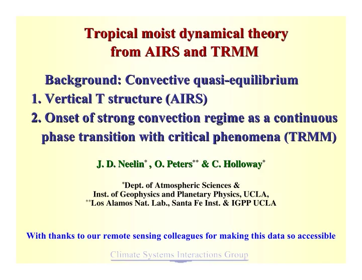
Tropical moist dynamical theory Tropical moist dynamical theory from AIRS and TRMM from AIRS and TRMM Background: Convective quasi-equilibrium Background: Convective quasi-equilibrium 1. Vertical T structure (AIRS) 1. Vertical T structure (AIRS) 2. Onset of strong convection regime as a continuous 2. Onset of strong convection regime as a continuous phase transition with critical phenomena (TRMM) phase transition with critical phenomena (TRMM) O. Peters , * , ** * J. D. Neelin * O. Peters ** & C. Holloway & C. Holloway * J. D. Neelin * Dept. of Atmospheric Sciences & Inst. of Geophysics and Planetary Physics, UCLA, ** Los Alamos Nat. Lab., Santa Fe Inst. & IGPP UCLA With thanks to our remote sensing colleagues for making this data so accessible

Background: Convective Quasi-equilibrium (QE) Background: Convective Quasi-equilibrium (QE) Arakawa & Schubert 1974 ; Manabe et al 1965; Arakawa & Schubert 1974 Moorthi & Suarez 1992; Randall & Pan 1993; … • Posit that bulk effects of convection tend to establish statistical equilibrium among buoyancy-related fields – temperature T & moisture q • Slow driving (moisture convergence & evaporation, radiative cooling, …) by large scales generates conditional instability • Fast removal of buoyancy by moist convective up/down-drafts • Above onset threshold, strong convection/precip. increase to keep system close to onset • Convection tends to constrain vertical structure of T, q fields and T-q relationships

Quasi-equilibrium (QE) moist convection schemes (cont.) Quasi-equilibrium (QE) moist convection schemes (cont.) e.g., Smoothly posed convective adjustment Convective heating: (Betts 1986; Betts & Miller 1986) Q c = ( T c − T )/ τ c (if vert int > 0) Convective moisture sink (vertical integral=Precip): − Q q = ( q − q c )/ τ c (if vert int > 0) τ c time scale of convective adjustment T c convective temp. profile; may interact with atm boundary layer (ABL) moist static energy, tropospheric moisture T c ~ moist adiabat if neglect entrainment,… q c = α q sat ( T ) convective moisture closure T c incl. ABL adjustment by downdrafts to satisfy energy constraint: vertically integrated ( Q c + Q q )=0 Later: vert int ( q)=w , and we’ll look for w c

1. Tropical vertical T structure 1. Tropical vertical T structure C. Holloway & J. D. Neelin, in prep for J. Atmos. C. Holloway & J. D. Neelin, in prep for J. Atmos. Sci Sci. . • Background: implications of convective quasi-equilibrium • QE postulates deep convection constrains vertical structure of temperature through troposphere near convection • If so, gives vertical str. of baroclinic geopotential variations, wind • On what space/time scales does this hold well? • Approx. moist adiabat? Relation to ABL? Top? *

Vertical Temperature structure Vertical Temperature structure (Rawinsondes avgd for 3 trop W Pacific stations) Monthly T regression coeff. of each Correlation coeff. level on 850-200mb avg T. • CARDS monthly 1953-1999 anomalies, shading < 5% signif. • Curve for moist adiabatic vertical structure in red.

Vertical Temperature structure Vertical Temperature structure Monthly T regression coeff. of each level on 850-200mb avg T. CARDS Rawinsondes avgd for 3 trop Western Pacific stations, 1953-99 AIRS monthly (avg for similar Western Pacific box, 2003-2005) • shading < 5% signif. • Curve for moist adiabatic vertical structure in red.

Vertical Temperature structure Vertical Temperature structure (Daily, as function of spatial scale) AIRS daily T (a) Regression of T at each level on 850-200mb avg T For 4 spatial averages, from all-tropics to 2.5 degree box Red curve corresp to moist adiabat. (b) Correlation of T(p) to 850-200mb avg T • AIRS level 2 v4 daily avg Nov 2003-Nov 2005

Vertical Temperature structure Vertical Temperature structure (and implied baroclinic geopotential structure) AIRS daily T regressed on 850- Resulting baroclinic 200mb avg T vs. moist adiabat. geopotential • AIRS level 2 v3 daily avg Jun-Jul 2003, markers signif. at 5%. All tropics = 15S-15N; Pac. Warm pool= 10S-10N, 140-180E.

QE in climate models QE in climate models (HadCM3, ECHAM5, GFDL CM2.1) (HadCM3, ECHAM5, GFDL CM2.1) Monthly T anoms regressed on Model global warming T 850-200mb T vs. moist adiabat. profile response • Regression on 1970-1994 of IPCC AR4 20 th C runs, markers signif. at 5%. Pac. Warm pool= 10S-10N, 140-180E. Response to SRES A2 for 2070-2094 minus 1970-1994 (htpps://esg.llnl.gov).

2. Onset of strong convection regime as a continuous 2. Onset of strong convection regime as a continuous phase transition with critical phenomena phase transition with critical phenomena J. D. Neelin, in prep for TBD. O. Peters & J. D. Neelin, in prep for TBD. O. Peters & • Background: precip tends to increase with column water vapor at >daily time scales (e.g., Bretherton et al 2004) • What happens at strong precip? Half of convective events in 6 min. station data are > 20 mm/hr. (Jones & Smith 1978) • In models, convection onsets when moisture large enough to create conditional instability & buoyant plumes for a given T • Convective QE postulates sound similar to self-organized criticality postulates, known in stat. mech. models to be assoc. with continuous phase transitions (NB. Not to be confused with the first order phase transition of condensation at microphysical scales) • Data here: Tropical Rainfall Measuring Mission (TRMM) microwave imager (TMI) water vapor, precip/cloud liquid water from Remote Sensing Systems • In progress: AMSR-E, TRMM Precip radar (2B31 product)

Western Pacific precip precip vs vs column water vapor column water vapor Western Pacific • Tropical Rainfall Measuring Mission Microwave Imager (TMI) data Western Pacific • Wentz & Spencer (1998) algorithm Eastern Pacific • Average precip P(w) in each 0.3 mm w bin (typically 10 4 to 10 7 counts per bin in 5 yrs) • 0.25 degree resolution • No explicit time averaging

Indian Ocean for SST within 1C bin at 25 25C C Indian Ocean for SST within 1C bin at Power law fit: P(w)=a(w-w c ) β

Indian Ocean for SST within 1C bin at 31 31C C Indian Ocean for SST within 1C bin at Power law fit: P(w)=a(w-w c ) β

Oslo model Oslo model (stochastic lattice model motivated by rice pile avalanches) (stochastic lattice model motivated by rice pile avalanches) [NB: not suggesting Oslo model applies to moist convection. Just an example of some generic properties common to many systems.] • Frette et al (Nature, 1996) • Christensen et al (Phys. Res. Lett., 1996; Phys. Rev. E. 2004)

Things to expect from continuous phase transition Things to expect from continuous phase transition critical phenomena critical phenomena • Behavior approaches P ( w )= a ( w-w c ) β above transition • exponent β should be robust in different regions, conditions. ("universality" for given class of model, variable) • critical value w c should depend on other conditions: region, boundary layer T , q (TMI SST as proxy), tropospheric temperature,... • factor a also non-universal; re-scaling P and w should collapse curves for different regions • below transition, expect P ( w ) depends on finite size effects. Spatial avg over length L increases # of degrees of freedom in the average.

Things to expect (cont.) Things to expect (cont.) • Precip variance σ P ( w ) should become large at critical point. • Expect L 2 σ P ( w,L ) ∝ L γ / ν near the critical region • i.e., spatial correlation becomes long (power law) near crit. point • Here check effects of spatial averaging length L . Can one collapse curves for σ P ( w ) in critical region? • correspondence of self-organized criticality in an open (dissipative), slowly driven) system, to the absorbing state phase transition of a corresponding (closed, no drive) system. • frequency of occurrence: expect maximum just below w c • Refs: e.g., Yeomans (1996; Stat. Mech. of Phase transitions, Oxford UP), Vespignani & Zapperi (Phys. Rev. Lett, 1997), Christensen et al (Phys. Rev. E, 2004)

log-log Precip Precip. . vs vs ( (w-w w-w c ) log-log c ) • Slope of each line ( β ) = 0.215 Eastern Pacific shifted for clarity Western Pacific Atlantic ocean Indian ocean (individual fits to β within ± 0.02)

How well do the curves collapse when rescaled? How well do the curves collapse when rescaled? • Original Western Pacific Eastern Pacific

How well do the curves collapse when rescaled? How well do the curves collapse when rescaled? • Rescale w and P by i i factors f p , f w for each region i Western Pacific Eastern Pacific

Collapse of Precip Precip. & . & Precip Precip. variance for . variance for Collapse of different regions different regions • Slope of each line ( β ) = 0.215 Variance Eastern Pacific Western Pacific Precip Atlantic ocean Indian ocean Western Pacific Eastern Pacific

Western Pacific for SST within 1C bin of 30C Western Pacific for SST within 1C bin of 30C Frequency of occurrence All cases Precip Frequency of occurrence Precipitating

TMI column water vapor and Precipitation TMI column water vapor and Precipitation Western Pacific example Western Pacific example

TMI column water vapor and Precipitation TMI column water vapor and Precipitation Atlantic example Atlantic example