Day 2: Linear Regression and Statistical Learning Lucas Leemann - PowerPoint PPT Presentation

�� Day 2: Linear Regression and Statistical Learning Lucas Leemann Essex Summer School Introduction to Statistical Learning L. Leemann (Essex Summer School) Day 2 Introduction to SL 1 / 53

�� Day 2 Outline 1 Simple linear regression Estimation of the parameters Confidence intervals Hypothesis testing Assessing overall accuracy of the model Multiple Linear Regression Interpretation Model fit 2 Qualitative predictors Qualitative predictors in regression models Interactions 3 Comparison of KNN and Regression L. Leemann (Essex Summer School) Day 2 Introduction to SL 2 / 53

�� Simple linear regression L. Leemann (Essex Summer School) Day 2 Introduction to SL 3 / 53

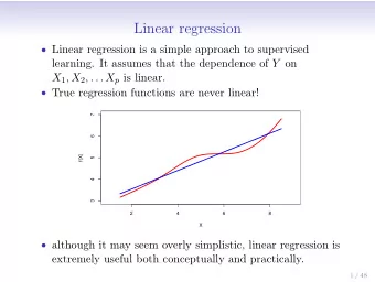
�� • Linear regression is a simple approach to supervised learning. It assumes that the dependence of Y on X 1 , X 2 , . . . , X p is linear. • True regression functions are never linear! • Although it may seem overly simplistic, linear regression is extremely useful both conceptually and practically. L. Leemann (Essex Summer School) Day 2 Introduction to SL 4 / 53

�� Linear regression for the advertising data Consider the advertising data. Questions we might ask: • Is there a relationship between advertising budget and sales? • How strong is the relationship between advertising budget and sales? • Which media contribute to sales? • How accurately can we predict future sales? • Is the relationship linear? • Is there synergy among the advertising media? L. Leemann (Essex Summer School) Day 2 Introduction to SL 5 / 53

�� Advertising data 25 25 25 20 20 20 Sales Sales Sales 15 15 15 10 10 10 5 5 5 0 50 100 200 300 0 10 20 30 40 50 0 20 40 60 80 100 TV Radio Newspaper L. Leemann (Essex Summer School) Day 2 Introduction to SL 6 / 53

�� Simple linear regression using a single predictor X • We assume a model Y = � 0 + � 1 X + ✏ , where � 0 and � 1 are two unknown constants that represent the intercept and slope, also known as coe ffi cients or parameters, and ✏ is the error term. • Given some estimates ˆ � 0 and ˆ � 1 for the model coe ffi cients, we predict future sales using y = ˆ � 0 + ˆ ˆ � 1 x , where ˆ y indicates a prediction of Y on the basis of X = x . The hat symbol denotes an estimated value. L. Leemann (Essex Summer School) Day 2 Introduction to SL 7 / 53

�� Estimation of the parameters by least squares y i = ˆ � 0 + ˆ • Let ˆ � 1 x i be the prediction for Y based on the i th value of X . Then e i = y i � ˆ y i represents the i th residual. • We define the residual sum of squares (RSS) as RSS = e 2 1 + e 2 2 + · · · + e 2 n , or equivalently as RSS = ( y 1 � ˆ � 0 � ˆ � 1 x 1 ) 2 +( y 2 � ˆ � 0 � ˆ � 1 x 2 ) 2 + · · · +( y n � ˆ � 0 � ˆ � 1 x n ) 2 . L. Leemann (Essex Summer School) Day 2 Introduction to SL 8 / 53

�� Estimation of the parameters by least squares • The least squares approach chooses ˆ � 0 and ˆ � 1 to minimize the RSS. The minimizing values can be shown to be P n i =1 ( x i � ¯ x )( y i � ¯ y ) ˆ � 1 = , P n i =1 ( x i � ¯ x ) 2 ˆ y � ˆ � 0 = ¯ � 1 ¯ x , P n P n y ⌘ 1 x ⌘ 1 where ¯ i =1 y i and ¯ i =1 x i are the sample means. n n L. Leemann (Essex Summer School) Day 2 Introduction to SL 9 / 53

�� Example: advertising data 25 20 Sales 15 10 5 0 50 100 150 200 250 300 TV The least squares fit for the regression of sales on TV. The fit is found by minimizing the sum of squared residuals. In this case a linear fit captures the essence of the relationship, although it is somewhat deficient in the left of the plot. L. Leemann (Essex Summer School) Day 2 Introduction to SL 10 / 53

�� Assessing the Accuracy of the Coe ffi cient Estimates • The standard error of an estimator reflects how it varies under repeated sampling. We have � 2 � 1 ) 2 = SE (ˆ x ) 2 , P n i =1 ( x i � ¯ x 2  1 ¯ � � 0 ) 2 = � 2 SE (ˆ n + , P n x ) 2 i =1 ( x i � ¯ where � 2 = Var ( ✏ ) • These standard errors can be used to compute confidence intervals. A 95% confidence interval is defined as a range of values such that with 95% probability, the range will contain the true unknown value of the parameter. It has the form � 1 ± 2 ⇥ SE (ˆ ˆ � 1 ) . L. Leemann (Essex Summer School) Day 2 Introduction to SL 11 / 53

�� Confidence Intervals That is, there is approximately a 95% chance that the interval  � � 1 � 2 ⇥ SE (ˆ ˆ � 1 ) , ˆ � 1 + 2 ⇥ SE (ˆ � 1 ) will contain the true value of � 1 (under a scenario where we got repeated samples like the present sample). L. Leemann (Essex Summer School) Day 2 Introduction to SL 12 / 53

�� Hypothesis testing • Standard errors can also be used to perform hypothesis tests on the coe ffi cients. The most common hypothesis test involves testing the null hypothesis of H 0 : There is no relationship between X and Y versus the alternative hypothesis. H A : There is some relationship between X and Y . • Mathematically, this corresponds to testing versus H 0 : � 1 = 0 versus H A : � 1 6 = 0 , since if � 1 = 0 then the model reduces to Y = � 0 + ✏ , and X is not associated with Y . L. Leemann (Essex Summer School) Day 2 Introduction to SL 13 / 53

�� Hypothesis testing • To test the null hypothesis, we compute a t-statistic, given by ˆ � 1 � 0 t = , SE (ˆ � 1 ) • This will have a t-distribution with n � 2 degrees of freedom, assuming � 1 = 0. • Using statistical software, it is easy to compute the probability of observing any value equal to | t | or larger. We call this probability the p-value. L. Leemann (Essex Summer School) Day 2 Introduction to SL 14 / 53

�� Assessing the Overall Accuracy of the Model • We compute the Residual Standard Error v n r u 1 1 X u y i ) 2 , RSE = n � 2 RSS = ( y i � ˆ t n � 2 i =1 where the residual sum-of-squares is RSS = P n y i ) 2 . i =1 ( y i � ˆ • R-squared or fraction of variance explained is R 2 = TSS � RSS = 1 � RSS TSS TSS y ) 2 is the total sum of squares. where TSS = P n i =1 ( y i � ¯ L. Leemann (Essex Summer School) Day 2 Introduction to SL 15 / 53

�� Results for the advertising data L. Leemann (Essex Summer School) Day 2 Introduction to SL 16 / 53

�� Results for the advertising data L. Leemann (Essex Summer School) Day 2 Introduction to SL 17 / 53

�� Multiple Linear Regression • Here our model is Y = � 0 + � 1 X 1 + � 2 X 2 + · · · + � p X p + ✏ , • We interpret � j as the average e ff ect on Y of a one unit increase in X j , holding all other predictors fixed. In the advertising example, the model becomes sales = � 0 + � 1 ⇥ TV + � 2 ⇥ radio + � p ⇥ newspaper + ✏ . L. Leemann (Essex Summer School) Day 2 Introduction to SL 18 / 53

�� Interpreting regression coe ffi cients • The ideal scenario is when the predictors are uncorrelated – a balanced design: • Each coe ffi cient can be estimated and tested separately. • Interpretations such as “a unit change in X j is associated with a � j change in Y , while all the other variables stay fixed”, are possible. • Correlations amongst predictors cause problems: • The variance of all coe ffi cients tends to increase, sometimes dramatically • Interpretations become hazardous – when X j changes, everything else changes. • Claims of causality are di ffi cult to justify with observational data. L. Leemann (Essex Summer School) Day 2 Introduction to SL 19 / 53

�� The woes of (interpreting) regression coe ffi cients “Data Analysis and Regression” Mosteller and Tukey 1977 • a regression coe ffi cient � j estimates the expected change in Y per unit change in X j , with all other predictors held fixed. But predictors usually change together! • Example: Y total amount of change in your pocket; X 1 = number of coins; X 2 = number of pennies, nickels and dimes. By itself, regression coe ffi cient of Y on X 2 will be > 0. But how about with X 1 in model? • Y = number of tackles by a rugby player in a season; W and H are his weight and height. Fitted regression model is Y = � 0 + . 50 W � . 10 H . How do we interpret ˆ ˆ � 2 < 0? L. Leemann (Essex Summer School) Day 2 Introduction to SL 20 / 53

�� Two quotes by famous Statisticians • “Essentially, all models are wrong, but some are useful” George Box • “The only way to find out what will happen when a complex system is disturbed is to disturb the system, not merely to observe it passively” Fred Mosteller and John Tukey, paraphrasing George Box L. Leemann (Essex Summer School) Day 2 Introduction to SL 21 / 53

�� Estimation and Prediction for Multiple Regression • Given estimates ˆ � 0 , ˆ � 1 , . . . , ˆ � p , we can make predictions using the formula y = ˆ � 0 + ˆ � 1 x 1 + ˆ � 2 x 2 + · · · + ˆ ˆ � p x p . • We estimate � 0 , � 1 , . . . , � p as the values that minimize the sum of squared residuals n n y i ) 2 = X X ( y i � ˆ � 0 � ˆ � 1 x i 1 � ˆ � 2 x i 2 � · · · � ˆ � p x ip ) 2 . RSS = ( y i � ˆ i =1 i =1 This is done using standard statistical software. The values � 0 , ˆ ˆ � 1 , . . . , ˆ � p that minimize RSS are the multiple least squares regression coe ffi cient estimates. L. Leemann (Essex Summer School) Day 2 Introduction to SL 22 / 53