DATABASE SYSTEM IMPLEMENTATION GT 4420/6422 // SPRING 2019 // - PowerPoint PPT Presentation
DATABASE SYSTEM IMPLEMENTATION GT 4420/6422 // SPRING 2019 // @JOY_ARULRAJ LECTURE #20: PARALLEL JOIN ALGORITHMS (HASHING) 2 ANATOMY OF A DATABASE SYSTEM Process Manager Connection Manager + Admission Control Query Parser Query Processor
38 RADIX PARTITIONING Scan the input relation multiple times to generate the partitions. Multi-step pass over the relation: → Step #1: Scan R and compute a histogram of the # of tuples per hash key for the radix at some offset. → Step #2: Use this histogram to determine output offsets by computing the prefix sum . → Step #3: Scan R again and partition them according to the hash key.
39 RADIX The radix is the value of an integer at a particular position (using its base). Input 89 12 23 08 41 64
40 RADIX The radix is the value of an integer at a particular position (using its base). Input 89 12 23 08 41 64
41 RADIX The radix is the value of an integer at a particular position (using its base). Input 89 12 23 08 41 64 Radix 9 2 3 8 1 4
42 RADIX The radix is the value of an integer at a particular position (using its base). Input 89 12 23 08 41 64 Radix
43 RADIX The radix is the value of an integer at a particular position (using its base). Input 89 12 23 08 41 64 Radix 8 1 2 0 4 6
44 PREFIX SUM The prefix sum of a sequence of numbers ( x 0 , x 1 , … , x n ) is a second sequence of numbers ( y 0 , y1, … , y n ) that is a running total of the input sequence. Input 1 2 3 4 5 6
45 PREFIX SUM The prefix sum of a sequence of numbers ( x 0 , x 1 , … , x n ) is a second sequence of numbers ( y 0 , y1, … , y n ) that is a running total of the input sequence. Input 1 2 3 4 5 6 Prefix Sum 1
46 PREFIX SUM The prefix sum of a sequence of numbers ( x 0 , x 1 , … , x n ) is a second sequence of numbers ( y 0 , y1, … , y n ) that is a running total of the input sequence. Input 1 2 3 4 5 6 + Prefix Sum 1
47 PREFIX SUM The prefix sum of a sequence of numbers ( x 0 , x 1 , … , x n ) is a second sequence of numbers ( y 0 , y1, … , y n ) that is a running total of the input sequence. Input 1 2 3 4 5 6 + Prefix Sum 1 3
48 PREFIX SUM The prefix sum of a sequence of numbers ( x 0 , x 1 , … , x n ) is a second sequence of numbers ( y 0 , y1, … , y n ) that is a running total of the input sequence. Input 1 2 3 4 5 6 + + + + + Prefix Sum 1 3 6 10 15 21
49 RADIX PARTITIONS # 0 7 p # 1 8 p 0 # 1 9 hash P (key) p # 0 7 p # 0 3 p # 1 1 p 1 # 1 5 p # 1 0 p Source: Spyros Blanas
50 RADIX PARTITIONS Step #1: Inspect input, create histograms # 0 7 p # 1 8 p 0 # 1 9 hash P (key) p # 0 7 p # 0 3 p # 1 1 p 1 # 1 5 p # 1 0 p Source: Spyros Blanas
51 RADIX PARTITIONS Step #1: Inspect input, create histograms # 0 7 p # 1 8 p 0 # 1 9 hash P (key) p # 0 7 p # 0 3 p # 1 1 p 1 # 1 5 p # 1 0 p Source: Spyros Blanas
52 RADIX PARTITIONS Step #1: Inspect input, create histograms # 0 7 p # 1 8 p 0 # 1 9 hash P (key) p # 0 7 p # 0 3 p # 1 1 p 1 # 1 5 p # 1 0 p Source: Spyros Blanas
53 RADIX PARTITIONS Step #1: Inspect input, create histograms # 0 7 p # 1 8 p 0 # 1 9 hash P (key) p # 0 7 p # 0 3 p # 1 1 p 1 # 1 5 p # 1 0 p Source: Spyros Blanas
54 RADIX PARTITIONS Step #1: Inspect input, create histograms # 0 7 p # 1 8 p 0 # 1 9 hash P (key) p # 0 7 p # 0 3 p # 1 1 p 1 # 1 5 p # 1 0 p Source: Spyros Blanas
55 RADIX PARTITIONS Step #1: Inspect input, create histograms # 0 7 p # 1 8 p 0 # 1 9 hash P (key) p Partition 0: 2 # 0 7 Partition 1: 2 p # 0 3 p # 1 1 p 1 # 1 5 p Partition 0: 1 # 1 0 Partition 1: 3 p Source: Spyros Blanas
56 RADIX PARTITIONS Step #2: Compute output offsets # 0 7 p # 1 8 p 0 # 1 9 hash P (key) p Partition 0: 2 # 0 7 Partition 1: 2 p # 0 3 p # 1 1 p 1 # 1 5 p Partition 0: 1 # 1 0 Partition 1: 3 p Source: Spyros Blanas
57 RADIX PARTITIONS Step #2: Compute output offsets Partition 0 , CPU 0 # 0 7 p # 1 8 p 0 Partition 0, CPU 1 # 1 9 hash P (key) p Partition 0: 2 Partition 1 , CPU 0 # 0 7 Partition 1: 2 p # 0 3 p Partition 1, CPU 1 # 1 1 p 1 # 1 5 p Partition 0: 1 # 1 0 Partition 1: 3 p Source: Spyros Blanas
58 RADIX PARTITIONS Step #3: Read input and partition Partition 0 , CPU 0 # 0 7 p # 1 8 p 0 Partition 0, CPU 1 # 1 9 hash P (key) p Partition 0: 2 Partition 1 , CPU 0 # 0 7 Partition 1: 2 p # 0 3 p Partition 1, CPU 1 # 1 1 p 1 # 1 5 p Partition 0: 1 # 1 0 Partition 1: 3 p Source: Spyros Blanas
59 RADIX PARTITIONS Step #3: Read input and partition Partition 0 , CPU 0 # 0 7 0 7 p # 1 8 p 0 Partition 0, CPU 1 # 1 9 0 3 hash P (key) p Partition 0: 2 Partition 1 , CPU 0 # 0 7 Partition 1: 2 p # 0 3 p Partition 1, CPU 1 # 1 1 p 1 # 1 5 p Partition 0: 1 # 1 0 Partition 1: 3 p Source: Spyros Blanas
60 RADIX PARTITIONS Step #3: Read input and partition Partition 0 , CPU 0 # 0 7 0 7 p # 1 8 0 7 p 0 Partition 0, CPU 1 # 1 9 0 3 hash P (key) p Partition 0: 2 Partition 1 , CPU 0 # 0 7 1 8 Partition 1: 2 p # 0 3 1 9 p Partition 1, CPU 1 # 1 1 1 1 p 1 # 1 5 1 5 p Partition 0: 1 # 1 0 1 0 Partition 1: 3 p Source: Spyros Blanas
61 RADIX PARTITIONS Partition 0 # 0 7 0 7 p # 1 8 0 7 p 0 # 1 9 0 3 hash P (key) p Partition 0: 2 Partition 1 # 0 7 1 8 Partition 1: 2 p # 0 3 1 9 p # 1 1 1 1 p 1 # 1 5 1 5 p Partition 0: 1 # 1 0 1 0 Partition 1: 3 p Source: Spyros Blanas
62 RADIX PARTITIONS Recursively repeat until target number of partitions have been created Partition 0 # 0 7 0 7 p # 1 8 0 7 p 0 # 1 9 0 3 hash P (key) p Partition 0: 2 Partition 1 # 0 7 1 8 Partition 1: 2 p # 0 3 1 9 p # 1 1 1 1 p 1 # 1 5 1 5 p Partition 0: 1 # 1 0 1 0 Partition 1: 3 p Source: Spyros Blanas
63 RADIX PARTITIONS Recursively repeat until target number of partitions have been created # 0 7 0 7 p # 1 8 0 7 p 0 0 # 1 9 0 3 hash P (key) p Partition 0: 2 # 0 7 1 8 Partition 1: 2 p # 0 3 1 9 p # 1 1 1 1 p 1 1 # 1 5 1 5 p Partition 0: 1 # 1 0 1 0 Partition 1: 3 p Source: Spyros Blanas
64 RADIX PARTITIONS Recursively repeat until target number of partitions have been created # 0 7 0 7 p # 1 8 0 7 p 0 0 # 1 9 0 3 hash P (key) p Partition 0: 2 # 0 7 1 8 Partition 1: 2 p # 0 3 1 9 p # 1 1 1 1 p 1 1 # 1 5 1 5 p Partition 0: 1 # 1 0 1 0 Partition 1: 3 p Source: Spyros Blanas
65 RADIX PARTITIONS Recursively repeat until target number of partitions have been created # 0 7 0 7 p # 1 8 0 7 p 0 0 # 1 9 0 3 hash P (key) p Partition 0: 2 # 0 7 1 8 Partition 1: 2 p # 0 3 1 9 p # 1 1 1 1 p 1 1 # 1 5 1 5 p Partition 0: 1 # 1 0 1 0 Partition 1: 3 p Source: Spyros Blanas
66 BUILD PHASE The threads are then to scan either the tuples (or partitions) of R . For each tuple, hash the join key attribute for that tuple and add it to the appropriate bucket in the hash table. → The buckets should only be a few cache lines in size.
67 HASH TABLE Design Decision #1: Hash Function → How to map a large key space into a smaller domain. → Trade-off between being fast vs. collision rate. Design Decision #2: Hashing Scheme → How to handle key collisions after hashing. → Trade-off between allocating a large hash table vs. additional instructions to find/insert keys.
68 HASH FUNCTIONS We don’t want to use a cryptographic hash function for our join algorithm. We want something that is fast and will have a low collision rate.
69 HASH FUNCTIONS MurmurHash (2008) → Designed to a fast, general purpose hash function. Google CityHash (2011) → Based on ideas from MurmurHash2 → Designed to be faster for short keys (<64 bytes). Google FarmHash (2014) → Newer version of CityHash with better collision rates. CLHash (2016) → Fast hashing function based on carry-less multiplication.
70 HASH FUNCTION BENCHMARKS Intel Core i7-8700K @ 3.70GHz std::hash MurmurHash3 CityHash FarmHash CLHash 18000 Throughput (MB/sec) 12000 6000 0 1 51 101 151 201 251 Key Size (bytes) Source: Fredrik Widlund
71 HASH FUNCTION BENCHMARKS Intel Core i7-8700K @ 3.70GHz std::hash MurmurHash3 CityHash FarmHash CLHash 18000 64 32 192 Throughput (MB/sec) 128 12000 6000 0 1 51 101 151 201 251 Key Size (bytes) Source: Fredrik Widlund
72 HASH FUNCTION BENCHMARKS Intel Core i7-8700K @ 3.70GHz std::hash MurmurHash3 CityHash FarmHash CLHash 192 36000 128 Throughput (MB/sec) 24000 64 32 12000 0 1 51 101 151 201 251 Key Size (bytes) Source: Fredrik Widlund
73 HASHING SCHEMES Approach #1: Chained Hashing Approach #2: Linear Hashing Approach #3: Robin Hood Hashing Approach #4: Cuckoo Hashing
74 CHAINED HASHING Maintain a linked list of “buckets” for each slot in the hash table. Resolve collisions by placing all elements with the same hash key into the same bucket. → To determine whether an element is present, hash to its bucket and scan for it. → Insertions and deletions are generalizations of lookups.
75 CHAINED HASHING hash(key) Ø ⋮ ⋮
76 LINEAR HASHING Single giant table of slots. Resolve collisions by linearly searching for the next free slot in the table. → To determine whether an element is present, hash to a location in the table and scan for it. → Have to store the key in the table to know when to stop scanning. → Insertions are generalizations of lookups.
77 LINEAR HASHING hash(key) A B C D E F
78 LINEAR HASHING hash(key) A B | A hash(A) C D E F
79 LINEAR HASHING hash(key) | B hash(B) A B | A hash(A) C D E F
80 LINEAR HASHING hash(key) | B hash(B) A B | A hash(A) C D E F
81 LINEAR HASHING hash(key) | B hash(B) A B | A hash(A) C | C hash(C) D E F
82 LINEAR HASHING hash(key) | B hash(B) A B | A hash(A) C | C hash(C) D | D E hash(D) F
83 LINEAR HASHING hash(key) | B hash(B) A B | A hash(A) C | C hash(C) D | D E hash(D) F
84 LINEAR HASHING hash(key) | B hash(B) A B | A hash(A) C | C hash(C) D | D E hash(D) F | E hash(E)
85 LINEAR HASHING hash(key) | B hash(B) A B | A hash(A) C | C hash(C) D | D E hash(D) F | E hash(E) | F hash(F)
86 OBSERVATION To reduce the # of wasteful comparisons during the join, it is important to avoid collisions of hashed keys. This requires a chained hash table with ~2x the number of slots as the # of elements in R .
87 ROBIN HOOD HASHING Variant of linear hashing that steals slots from "rich" keys and give them to "poor" keys. → Each key tracks the number of positions they are from where its optimal position in the table. → On insert, a key takes the slot of another key if the first key is farther away from its optimal position than the second key. RO ROBIN N HOOD HASHING NG Foundations of Computer Science 1985
88 ROBIN HOOD HASHING hash(key) A B C D E F
89 ROBIN HOOD HASHING hash(key) A B | A [0] hash(A) C D E F
90 ROBIN HOOD HASHING hash(key) A B | A [0] # of "Jumps" From First Position hash(A) C D E F
91 ROBIN HOOD HASHING hash(key) A B | A [0] hash(A) C D E F
92 ROBIN HOOD HASHING hash(key) | B [0] hash(B) A B | A [0] hash(A) C D E F
93 ROBIN HOOD HASHING hash(key) | B [0] hash(B) A B | A [0] hash(A) A[0] == C[0] C D E F
94 ROBIN HOOD HASHING hash(key) | B [0] hash(B) A B | A [0] hash(A) A[0] == C[0] C | C [1] hash(C) D E F
95 ROBIN HOOD HASHING hash(key) | B [0] hash(B) A B | A [0] hash(A) C | C [1] C[1] > D[0] hash(C) D E F
96 ROBIN HOOD HASHING hash(key) | B [0] hash(B) A B | A [0] hash(A) C | C [1] C[1] > D[0] hash(C) D | D [1] E hash(D) F
97 ROBIN HOOD HASHING hash(key) | B [0] hash(B) A B | A [0] hash(A) C | C [1] hash(C) D | D [1] E hash(D) F
98 ROBIN HOOD HASHING hash(key) | B [0] hash(B) A B | A [0] hash(A) A[0] == E[0] C | C [1] hash(C) D | D [1] E hash(D) F
99 ROBIN HOOD HASHING hash(key) | B [0] hash(B) A B | A [0] hash(A) A[0] == E[0] C | C [1] C[1] == E[1] hash(C) D | D [1] E hash(D) F
100 ROBIN HOOD HASHING hash(key) | B [0] hash(B) A B | A [0] hash(A) A[0] == E[0] C | C [1] C[1] == E[1] hash(C) D | D [1] D[1] < E[2] E hash(D) F
Recommend
More recommend
Explore More Topics
Stay informed with curated content and fresh updates.

