Notes on Hashing Owen Jow Last updated May 05, 2018 This document - PDF document

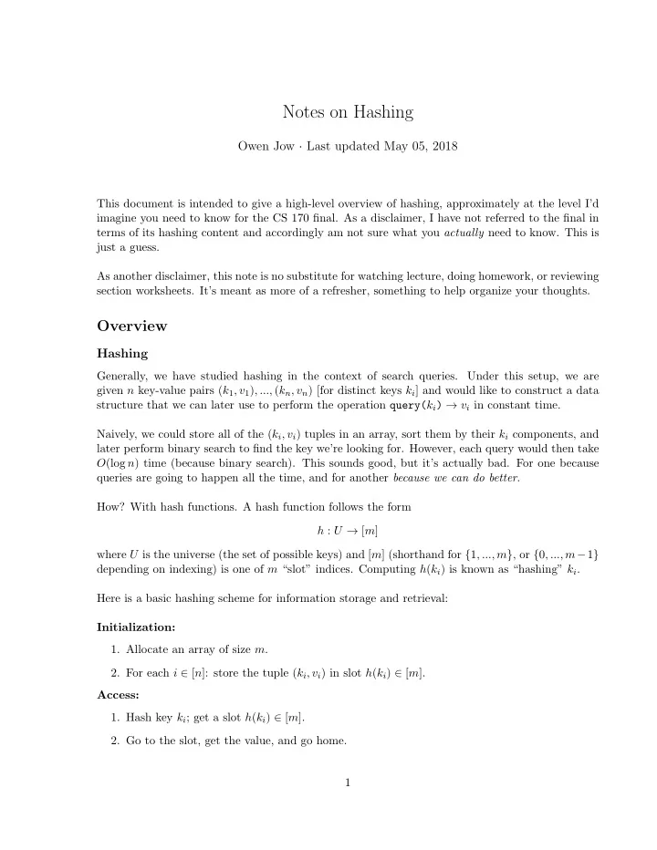
Notes on Hashing Owen Jow · Last updated May 05, 2018 This document is intended to give a high-level overview of hashing, approximately at the level I’d imagine you need to know for the CS 170 final. As a disclaimer, I have not referred to the final in terms of its hashing content and accordingly am not sure what you actually need to know. This is just a guess. As another disclaimer, this note is no substitute for watching lecture, doing homework, or reviewing section worksheets. It’s meant as more of a refresher, something to help organize your thoughts. Overview Hashing Generally, we have studied hashing in the context of search queries. Under this setup, we are given n key-value pairs ( k 1 , v 1 ) , ..., ( k n , v n ) [for distinct keys k i ] and would like to construct a data structure that we can later use to perform the operation query( k i ) → v i in constant time. Naively, we could store all of the ( k i , v i ) tuples in an array, sort them by their k i components, and later perform binary search to find the key we’re looking for. However, each query would then take O (log n ) time (because binary search). This sounds good, but it’s actually bad. For one because queries are going to happen all the time, and for another because we can do better . How? With hash functions. A hash function follows the form h : U → [ m ] where U is the universe (the set of possible keys) and [ m ] (shorthand for { 1 , ..., m } , or { 0 , ..., m − 1 } depending on indexing) is one of m “slot” indices. Computing h ( k i ) is known as “hashing” k i . Here is a basic hashing scheme for information storage and retrieval: Initialization: 1. Allocate an array of size m . 2. For each i ∈ [ n ]: store the tuple ( k i , v i ) in slot h ( k i ) ∈ [ m ]. Access: 1. Hash key k i ; get a slot h ( k i ) ∈ [ m ]. 2. Go to the slot, get the value, and go home. 1

Figure 1: basic hashing. In each slot we store a linked list of ( k i , v i ) tuples. In this scheme, each access time consists of the time it takes to evaluate h ( k i ) plus the time it takes to find ( k i , v i ) at slot h ( k i ). The former should be O (1). The latter depends on how many items are at slot h ( k i ), which in turn depends on the collisions our hash function creates. To assert an overall O (1) access time, we need to spread the data out as much as possible (avoid a bunch of collisions in any given slot)! Unfortunately, the following lemma exists: For every hash function, there exists a set of keys that are all mapped to the same slot. Note: this is assuming that the universe is sufficiently large. But it usually will be. For most inputs, our hash function might do pretty well. However, by this lemma there’s always an input that will make our hashing scheme useless (no better than storing everything in a list). And we want our search query algorithm to have guarantees for all inputs, not just random inputs. Thus, instead of hardcoding some h and using it, we will pick h at random as part of the algorithm. Specifically, we will pick h from a family of hash functions H . Assuming each h ∈ H performs well for most inputs, we will then have a good probability of getting a good h for the data we receive. Algorithm 1 No randomization 1: procedure h (k) Use black magic to turn k into a number from 1 to m 2: 3: procedure initialize (( k 1 , v 1 ) , ..., ( k n , v n )) Allocate an array of size m 4: For each i ∈ [ n ]: store the tuple ( k i , v i ) in slot h ( k i ) ∈ [ m ] 5: Algorithm 2 Randomization 1: procedure initialize (( k 1 , v 1 ) , ..., ( k n , v n )) h ← random h ∈ H 2: Allocate an array of size m 3: For each i ∈ [ n ]: store the tuple ( k i , v i ) in slot h ( k i ) ∈ [ m ] 4: Without randomization, there is surely an input (i.e. a bunch of ( k i , v i ) pairs) that will defeat us. With randomization, there is no such input. 2

1 As it happens, if the probability of a collision between any two distinct keys is ≤ m for a hash function chosen uniformly randomly from H , the expected number of collisions per slot is ≤ n m . n : the number of ( k i , v i ) pairs we’re hashing m : the number of slots we’re hashing to This is a great result – if n = m the expected number of collisions per slot is ≤ 1 – so let’s make sure H meets this condition. Such a hash family is called universal . Universal Hashing Formally, a family of hash functions H is universal if for all k 1 � = k 2 ∈ U , h ∈H [ h ( k 1 ) = h ( k 2 )] ≤ 1 Pr m Note: a simple universal hash family is the set of all functions from U to [ m ]. However, to store a generic random function from U to [ m ] would require | U | log m bits (because we would have to encode all of the mappings). Furthermore, to sample one of these functions we would need to randomize | U | log m bits. Since | U | is often massive, this is just too expensive. We should find a smaller universal hash family to sample from. For example, the family of key-indexed inner product functions seen in lecture. Our hashing scheme has now become Algorithm 3 Universal Hashing 1: h ← null 2: procedure initialize (( k 1 , v 1 ) , ..., ( k n , v n )) h ← random h from universal hash family H 3: Allocate an array of size m 4: For each i ∈ [ n ]: store the tuple ( k i , v i ) in slot h ( k i ) ∈ [ m ] 5: 6: procedure query ( k i ) Go to slot h ( k i ) and find ( k i , v i ) 7: Return v i 8: With universal hashing, in expectation we will have a constant number of collisions in each slot – and therefore an expected constant access time overall! Best of all, this will work for all data (hence the “universal” moniker). Still, maybe we would like a stronger guarantee than just expectation. How about a worst-case guarantee? This is where perfect hashing makes its entrance. Perfect Hashing In perfect hashing, we guarantee zero collisions and thus constant access time in the worst case. There are multiple ways to achieve perfect hashing; I’ll cover the one we discussed in class. During the initialization step of our current universal hashing algorithm, ( k i , v i ) pairs are distributed over a hash table as depicted in Figure 2 (to give an example). 3

Figure 2: basic hashing re-illustrated. Instead of laying collisions out into a list, perfect hashing invokes another hash function which maps each slot’s elements into a second-level array. If the first-layer hash function maps l i elements into slot i , then the second-layer hash function h i : U → [ l 2 i ] for slot i will map these l i elements into an array of size l 2 i . Why l 2 i ? Because then the probability of collision will be low. To be clear, we first hash each element into a table of size m . Then we re-hash the elements in each slot into another, bigger hash table such that there are no collisions. The sizes of the second-level hash tables do not all have to be the same. Figure 3: perfect hashing. The length of each second-level hash table is the square of the length of the original linked list at the slot. All hash functions are sampled from universal families. The total size of the two-layer hash table will then be � m i =1 l 2 i , since we expand each of m slots to a size that is the square of the number of elements that are originally mapped into it. We would like � m i =1 l 2 i to be on the order O ( n ). 4

Overall, the algorithm comes together as follows: Algorithm 4 Perfect Hashing 1: procedure initialize (( k 1 , v 1 ) , ..., ( k n , v n )) h ← random h from universal hash family H 2: Hash each of the k i ’s; get a distribution l 1 , ..., l m 3: (Check that � m i =1 l 2 i < 100 · n ; if not, resample h and hash again) 4: for each slot j = 1 , ..., m do 5: h j ← random h from universal hash family H j 6: Use h j to hash every k i originally mapped to slot j 7: (Check that there are no collisions; if there are, resample h j and hash again) 8: Store each v i in slot h j ( k i ) in the second-layer table for slot j 9: 10: procedure query ( k i ) Return the value at h h ( k i ) ( k i ) 11: Note that if we do end up with collisions, we resample the hash function and try again. We continue in this way until we have zero collisions. Therefore zero collisions is guaranteed. The only question is “how long does it take to find hash functions that work?” But since we’re using universal hash functions and second-layer arrays of length l 2 i , it shouldn’t take too long; after all, the probability of choosing an h i with zero collisions is greater than 1 2 . Perfect hashing uses randomness to find good (indeed perfect) hash functions for the given data. Common Confusions Hashing • Why can’t we just map elements to the indices 1 , 2 , 3 , ... in order? – This spreads the items out, but doesn’t address the issue of search queries. Once items are stored, how do we access them again in constant time? How do you know which element goes with which index? – If your answer is “use a dictionary,” that doesn’t help since dictionaries are hash maps. You’d only end up adding a layer of indirection on top of the already-proposed solution. • Do we sample a different hash function every time we hash something? – We only sample the hash function once. Once we start mapping things, we need the mappings to stay the same – otherwise we might lose track of where the items are. • Does the hash function map all of the keys at once? – No, a hash function only maps one element at a time. In case you are confused by the notation h : { 1 , ..., p } → { 1 , ..., m } , it means we’re mapping a single element in the set { 1 , ..., p } to a single element in the set { 1 , ..., m } . 5