Lecture 8: Hashing I Lecture Overview Dictionaries and Python - PDF document

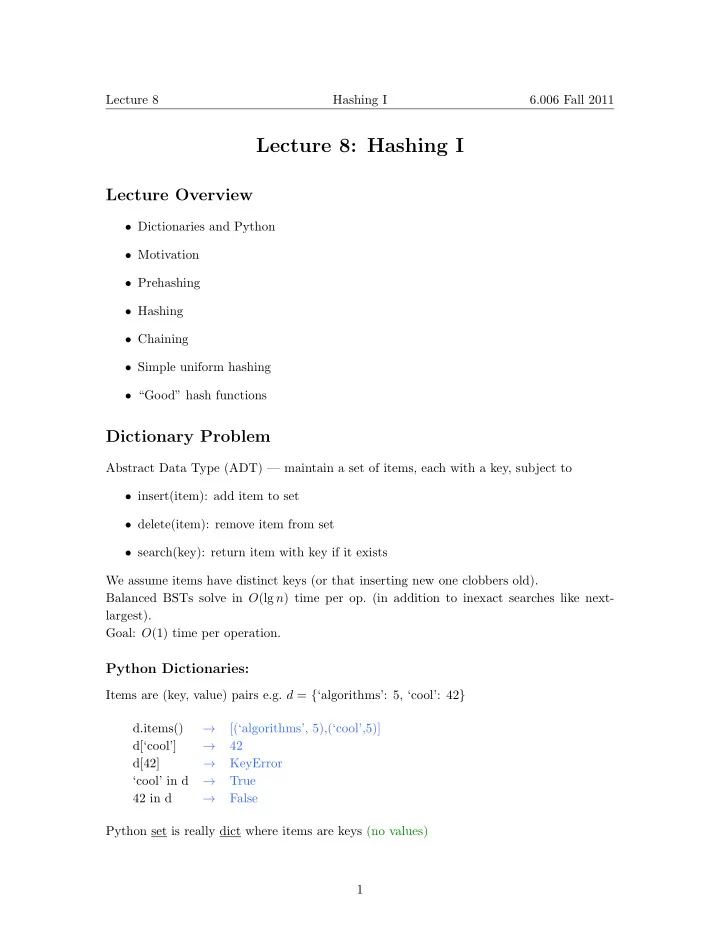
Lecture 8 Hashing I 6.006 Fall 2011 Lecture 8: Hashing I Lecture Overview • Dictionaries and Python • Motivation • Prehashing • Hashing • Chaining • Simple uniform hashing • “Good” hash functions Dictionary Problem Abstract Data Type (ADT) — maintain a set of items, each with a key, subject to • insert(item): add item to set • delete(item): remove item from set • search(key): return item with key if it exists We assume items have distinct keys (or that inserting new one clobbers old). Balanced BSTs solve in O (lg n ) time per op. (in addition to inexact searches like next- largest). Goal: O (1) time per operation. Python Dictionaries: Items are (key, value) pairs e.g. d = { ‘algorithms’: 5, ‘cool’: 42 } → d.items() [(‘algorithms’, 5),(‘cool’,5)] → d[‘cool’] 42 d[42] → KeyError ‘cool’ in d → True 42 in d → False Python set is really dict where items are keys (no values) 1

Lecture 8 Hashing I 6.006 Fall 2011 Motivation Dictionaries are perhaps the most popular data structure in CS • built into most modern programming languages (Python, Perl, Ruby, JavaScript, Java, C++, C#, . . . ) • e.g. best docdist code: word counts & inner product • implement databases: (DB HASH in Berkeley DB) – English word → definition (literal dict.) – English words: for spelling correction – word → all webpages containing that word – username → account object • compilers & interpreters: names → variables • network routers: IP address → wire • network server: port number → socket/app. • virtual memory: virtual address → physical Less obvious, using hashing techniques: • substring search (grep, Google) [L9] • string commonalities (DNA) [PS4] • file or directory synchronization (rsync) • cryptography: file transfer & identification [L10] How do we solve the dictionary problem? Simple Approach: Direct Access Table This means items would need to be stored in an array, indexed by key (random access) 2

Lecture 8 Hashing I 6.006 Fall 2011 0 1 2 key item key item item key . . . Figure 1: Direct-access table Problems: 1. keys must be nonnegative integers (or using two arrays, integers) ⇒ large space — e.g. one key of 2 256 is bad news. 2. large key range = 2 Solutions: Solution to 1 : “prehash” keys to integers. • In theory, possible because keys are finite = ⇒ set of keys is countable • In Python: hash(object) (actually hash is misnomer should be “prehash”) where object is a number, string, tuple, etc. or object implementing hash (default = id = memory address) • In theory, x = y ⇔ hash( x ) = hash( y ) • Python applies some heuristics for practicality: for example, hash(‘ \ 0 B ’) = 64 = hash(‘ \ 0 \ 0 C ’) • Object’s key should not change while in table (else cannot find it anymore) • No mutable objects like lists Solution to 2 : hashing (verb from French ‘hache’ = hatchet, & Old High German ‘happja’ = scythe) • Reduce universe U of all keys (say, integers) down to reasonable size m for table • idea: m ≈ n = # keys stored in dictionary • hash function h: U → { 0 , 1 , . . . , m − 1 } 3

Lecture 8 Hashing I 6.006 Fall 2011 T 0 k 1 1 . . . . . . U k . . k 3 h(k 1 ) = 1 1 k . . . .. k 2 k 4 k . 3 k 2 m-1 Figure 2: Mapping keys to a table • two keys k i , k j ∈ K collide if h ( k i ) = h ( k j ) How do we deal with collisions? We will see two ways 1. Chaining: TODAY 2. Open addressing: L10 Chaining Linked list of colliding elements in each slot of table . . . . . U k 1 k . k k k k 2 2 k 1 4 . 4 k 3 . h(k 1 ) = h(k 2 ) = k 3 h(k 4 ) Figure 3: Chaining in a Hash Table • Search must go through whole list T[h(key)] • Worst case: all n keys hash to same slot = ⇒ Θ( n ) per operation 4

Lecture 8 Hashing I 6.006 Fall 2011 Simple Uniform Hashing: An assumption (cheating): Each key is equally likely to be hashed to any slot of table, independent of where other keys are hashed. let n = # keys stored in table m = # slots in table load factor α = n/m = expected # keys per slot = expected length of a chain Performance This implies that expected running time for search is Θ(1+ α ) — the 1 comes from applying the hash function and random access to the slot whereas the α comes from searching the list. This is equal to O (1) if α = O (1), i.e., m = Ω( n ). Hash Functions We cover three methods to achieve the above performance: Division Method: h ( k ) = k mod m This is practical when m is prime but not too close to power of 2 or 10 (then just depending on low bits/digits). But it is inconvenient to find a prime number, and division is slow. Multiplication Method: h ( k ) = [( a · k ) mod 2 w ] ≫ ( w − r ) where a is random, k is w bits, and m = 2 r . This is practical when a is odd & 2 w − 1 < a < 2 w & a not too close to 2 w − 1 or 2 w . Multiplication and bit extraction are faster than division. 5

� Lecture 8 Hashing I 6.006 Fall 2011 w k a x 1 1 1 k k k } r Figure 4: Multiplication Method Universal Hashing [6.046; CLRS 11.3.3] For example: h ( k ) = [( ak + b ) mod p ] mod m where a and b are random ∈ { 0 , 1 , . . . p − 1 } , and p is a large prime ( > |U| ). This implies that for worst case keys k 1 = k 2 , (and for a, b choice of h ): 1 Pr a,b { event X k 1 k 2 } = Pr a,b { h ( k 1 ) = h ( k 2 ) } = m This lemma not proved here This implies that: � E a,b [# collisions with k 1 ] = E [ X k 1 k 2 ] k 2 � = E [ X k 1 k 2 ] k 2 � = Pr { X k 1 k 2 = 1 } � �� � k 2 1 m n = = α m This is just as good as above! 6

MIT OpenCourseWare http://ocw.mit.edu 6.006 Introduction to Algorithms Fall 2011 For information about citing these materials or our Terms of Use, visit: http://ocw.mit.edu/terms.

Lecture 9 Hashing II 6.006 Fall 2011 Lecture 9: Hashing II Lecture Overview • Table Resizing • Amortization • String Matching and Karp-Rabin • Rolling Hash Recall: Hashing with Chaining: collisions table all possible keys . . . . . k U 1 . k k k k 2 2 k 1 4 k . 4 k 3 h } . expected size n keys α = n/m m slots k 3 in set DS Figure 1: Hashing with Chaining Expected cost (insert/delete/search): Θ(1 + α ), assuming simple uniform hashing OR universal hashing & hash function h takes O (1) time. Division Method: h ( k ) = k mod m where m is ideally prime Multiplication Method: h ( k ) = [( a · k ) mod 2 w ] ≫ ( w − r ) where a is a random odd integer between 2 w − 1 and 2 w , k is given by w bits, and m = table size = 2 r . 1

Lecture 9 Hashing II 6.006 Fall 2011 How Large should Table be? • want m = Θ( n ) at all times • don’t know how large n will get at creation • m too small = ⇒ slow; m too big = ⇒ wasteful Idea: Start small (constant) and grow (or shrink) as necessary. Rehashing: To grow or shrink table hash function must change ( m, r ) = ⇒ must rebuild hash table from scratch for item in old table: → for each slot, for item in slot insert into new table = ⇒ Θ( n + m ) time = Θ( n ) if m = Θ( n ) How fast to grow? When n reaches m , say • m + =1? ⇒ rebuild every step = ⇒ n inserts cost Θ(1 + 2 + · · · + n ) = Θ( n 2 ) = • m ∗ =2? m = Θ( n ) still ( r + =1) ⇒ rebuild at insertion 2 i = = ⇒ n inserts cost Θ(1 + 2 + 4 + 8 + · · · + n ) where n is really the next power of 2 = Θ( n ) • a few inserts cost linear time, but Θ(1) “on average”. Amortized Analysis This is a common technique in data structures — like paying rent: $1500/month ≈ $50/day • operation has amortized cost T ( n ) if k operations cost ≤ k · T ( n ) • “ T ( n ) amortized” roughly means T ( n ) “on average”, but averaged over all ops. • e.g. inserting into a hash table takes O (1) amortized time. 2

Lecture 9 Hashing II 6.006 Fall 2011 Back to Hashing: Maintain m = Θ( n ) = ⇒ α = Θ(1) = ⇒ support search in O (1) expected time (assuming simple uniform or universal hashing) Delete: Also O (1) expected as is. • space can get big with respect to n e.g. n × insert, n × delete • solution: when n decreases to m/ 4, shrink to half the size = ⇒ O (1) amortized cost for both insert and delete — analysis is harder; see CLRS 17.4. Resizable Arrays: • same trick solves Python “list” (array) • = ⇒ list.append and list.pop in O (1) amortized 0 1 2 3 4 5 6 7 } } list unused Figure 2: Resizeable Arrays String Matching Given two strings s and t , does s occur as a substring of t ? (and if so, where and how many times?) E.g. s = ‘6.006’ and t = your entire INBOX (‘grep’ on UNIX) Simple Algorithm: any( s == t [ i : i + len(s)] for i in range(len( t ) − len( s ))) — O ( | s | ) time for each substring comparison = ⇒ O ( | s | · ( | t | − | s | )) time = O ( | s | · | t | ) potentially quadratic 3