Continuous time semi-Markov inference of biometric laws associated - PowerPoint PPT Presentation

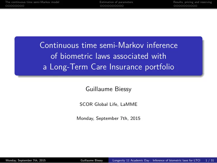
The continuous time semi-Markov model Estimation of parameters Results, pricing and reserving Continuous time semi-Markov inference of biometric laws associated with a Long-Term Care Insurance portfolio Guillaume Biessy SCOR Global Life, LaMME Monday, September 7th, 2015 Monday, September 7th, 2015 Guillaume Biessy Longevity 11 Academic Day : Inference of biometric laws for LTCI 1 / 31

The continuous time semi-Markov model Estimation of parameters Results, pricing and reserving High stakes Definition Dependency : permanent and consolidated state of inability to perform activities of daily living without someone else’s help. Phenomenon linked to ageing Multiple causes : cancer, dementia, neurological and cardiovascular diseases . . . Definition based on Activities of Daily Living (ADL) such as moving, clothing, bathing, feeding. Need to hire professional caregivers or join a nursing home. Associated costs up to 4 000 € a month in France. The French long-term care insurance market : First products appeared in the 1980s. Second market in the world, behind the US market. 7,3 M insured lives, 665 M € premium paid in 2014. Monday, September 7th, 2015 Guillaume Biessy Longevity 11 Academic Day : Inference of biometric laws for LTCI 2 / 31

The continuous time semi-Markov model Estimation of parameters Results, pricing and reserving Notation I A D For x 0 ě 0, let us consider a continuous-time process p Z x q x ě x 0 with values in the 3-state set E “ t A , I , D u of autonomy, dependency, death. Let us further assume that Z is cad-lag and that Z x 0 “ A and denote A x “ P p Z x “ A q , I x “ P p Z x “ I q , D x “ P p Z x “ D q . Hence A x 0 “ 1 and for all x ě x 0 , A x ` I x ` D x “ 1. Monday, September 7th, 2015 Guillaume Biessy Longevity 11 Academic Day : Inference of biometric laws for LTCI 3 / 31

The continuous time semi-Markov model Estimation of parameters Results, pricing and reserving Transition intensities I λ p x q µ i p x , t q A D µ a p x q The model is then defined using the transition intensities : 1 λ p x q “ lim h P p Z x ` h “ I | Z x “ A q h Ñ 0 1 µ a p x q “ lim h P p Z x ` h “ D | Z x “ A q h Ñ 0 1 µ i p x , t q “ lim h P p Z x ` t ` h “ D | Z x ´ “ A , Z x “ I , Z x ` t “ I q h Ñ 0 Monday, September 7th, 2015 Guillaume Biessy Longevity 11 Academic Day : Inference of biometric laws for LTCI 4 / 31

The continuous time semi-Markov model Estimation of parameters Results, pricing and reserving Evolution equations I λ p x q µ i p x , t q A D µ a p x q For x ě x 0 , t ě 0, we have ¨ ˛ ż x ˚ ‹ A x “ exp ˝ ´ r λ p u q ` µ a p u qs d u ‚ , x 0 ¨ ˛ ż x ż x ˝ ´ ‚ d u . I x “ λ p u q A u exp µ i p u , v ´ u q d v x 0 u Monday, September 7th, 2015 Guillaume Biessy Longevity 11 Academic Day : Inference of biometric laws for LTCI 5 / 31

The continuous time semi-Markov model Estimation of parameters Results, pricing and reserving Link with general mortality (1/2) I λ p x q µ i p x , t q t A , I u D µ g p x q A D µ a p x q Intensity of mortality for the general population : 1 µ g p x q “ lim h P p Z x ` h “ D | Z x P t A , I uq h Ñ 0 System of 3 differential equations : d d x A x “ ´r λ p x q ` µ a p x qs A x , (1) ¨ ˛ ż x ż x d ˝ ´ ‚ µ i p u , x ´ u q d u , d x I x “ λ p x q A x ´ λ p u q A u exp µ i p u , v ´ u q d v (2) x 0 u d d x p A x ` I x q “ ´ µ g p x qp A x ` I x q . (3) Monday, September 7th, 2015 Guillaume Biessy Longevity 11 Academic Day : Inference of biometric laws for LTCI 6 / 31

The continuous time semi-Markov model Estimation of parameters Results, pricing and reserving Link with general mortality (2/2) The following equation express the equivalence of forces of mortality ¨ ˛ ż x ż x ˝ ´ ‚ µ i p u , x ´ u q d u µ g p x qp A x ` I x q “ µ a p x q A x ` λ p u q A u exp µ i p u , v ´ u q d v x 0 u By denoting ∆ p x , t q “ µ i p x , t q ´ µ a p x ` t q and after a few lines of calculation, we get Mortality consistency equation ˜ ¸ x ş ş x λ p u q ∆ p u , x ´ u q exp ´ r ∆ p u , v ´ u q ´ λ p v qs d v d u x 0 u ˜ ¸ µ a p x q “ µ g p x q ´ . x ş x ş 1 ` λ p u q exp ´ r ∆ p u , v ´ u q ´ λ p v qs d v d u x 0 u Monday, September 7th, 2015 Guillaume Biessy Longevity 11 Academic Day : Inference of biometric laws for LTCI 7 / 31

The continuous time semi-Markov model Estimation of parameters Results, pricing and reserving Mixture model for dependent mortality (1/2) How to model dependent mortality ? Insurer’s experience shows very high death rates during the first few months spent in dependency. We believe this phenomenon can be explained by a strong heterogeneity among the dependent population, linked to causes of dependency. Causes like metastatic cancer, multiple stroke or severe cases of infarction are associated with very high death rates. Population structure therefore changes over time as individuals with higher mortality risks are among the first to die. Working assumption : dependent people can be separated in two populations, each with its own associated death rates. Monday, September 7th, 2015 Guillaume Biessy Longevity 11 Academic Day : Inference of biometric laws for LTCI 8 / 31

The continuous time semi-Markov model Estimation of parameters Results, pricing and reserving Mixture model for dependent mortality (2/2) I 1 µ i , 1 p x , t q λ 1 p x q A D µ a p x q λ 2 p x q µ i , 2 p x , t q I 2 Lemma Consider the above dependency model with two states I 1 and I 2 and let us assume that for x ě x 0 , t ě 0 and k P t 1 , 2 u , µ i , k p x , t q “ µ a p x ` t q ` ∆ k p x q . Then to ensure consistency with the 3-state model, the following relations must hold λ p x q “ λ 1 p x q ` λ 2 p x q ∆ 2 p x q ´ ∆ 1 p x q µ i p x , t q “ µ a p x ` t q ` ∆ 1 p x q ` 1 ` λ 1 p x q λ 2 p x q exp pr ∆ 2 p x q ´ ∆ 1 p x qs t q Monday, September 7th, 2015 Guillaume Biessy Longevity 11 Academic Day : Inference of biometric laws for LTCI 9 / 31

The continuous time semi-Markov model Estimation of parameters Results, pricing and reserving Data structure We assume contributors/annuitant databases containing the following variables : DoB : date of birth of the individual, DoS : date of start. For contributors, it is the date of subscribing. For annuitants, the date of entry in dependency. DoE and CoE : Date of end and cause of end for the individuals. Code 1 for death, 2 for entry in dependency, 0 for right-censoring. DoB DoS DoE CoE 23/12/1941 11/10/1992 27/09/2006 2 14/06/1926 28/03/1997 31/12/2013 0 17/04/1937 28/03/1995 04/08/2003 1 Table 1 : Example of a database of contributors. Estimation of parameters is then performed separately for men and women. Monday, September 7th, 2015 Guillaume Biessy Longevity 11 Academic Day : Inference of biometric laws for LTCI 10 / 31

The continuous time semi-Markov model Estimation of parameters Results, pricing and reserving Presentation of the portfolio Dependency based on a 3ADL4 definition, High volume portfolio, Data for higher ages (up to 95) and high duration in dependency (up to 13 years). Statistics Contributors Annuitants Number of lines 160 669 17 632 Person-year exposure 1 325 758 43 010 Observation period 10 years 19 years Censored trajectories 75,9 % 31,4 % Percentage of women 65,3 % 65,9 % Monday, September 7th, 2015 Guillaume Biessy Longevity 11 Academic Day : Inference of biometric laws for LTCI 11 / 31

The continuous time semi-Markov model Estimation of parameters Results, pricing and reserving Procedure for the estimation of biometric laws Logistic p Database of contributors λ Logistic µ a p 1 q x p semi-Markov ∆ Database of annuitants Equation µ a p 2 q x Mortality reference µ g p 2 q Brass x µ g p 1 q Database of insured lives Logistic x Figure 1 : Procedure for the estimation of biometric laws. Plain (resp. dashed) circle represents final (resp. intermediary) estimates of biometric laws. Monday, September 7th, 2015 Guillaume Biessy Longevity 11 Academic Day : Inference of biometric laws for LTCI 12 / 31

The continuous time semi-Markov model Estimation of parameters Results, pricing and reserving Intensity of incidence in dependency We consider a logistic form exp p a λ x ` b λ q λ p x q “ 1 ` exp p a λ x ` c λ q ` d λ with a λ ą 0, b λ , c λ P R and d λ ě 0. For an individual p defined by his/her age of entry in the portfolio x p ě 0, his/her age of exit y p ą x p and the associated exit cause c p P t 0 , 1 , 2 u the partial log-likelihood has the following expression y p ż l p p λ q “ δ 2 c p log p λ p y p qq ´ λ p u q d u x p ˆ ˙ ˆ 1 ` e a λ y p ` c λ ˙ e a λ y p ` b λ ´ e b λ ´ c λ “ δ 2 c p log 1 ` e a λ y p ` c λ ` d λ log ´ d λ p y p ´ x p q , 1 ` e a λ x p ` c λ a λ Monday, September 7th, 2015 Guillaume Biessy Longevity 11 Academic Day : Inference of biometric laws for LTCI 13 / 31