Chapter 8 Approximation Algorithms NEW CS 473: Theory II, Fall 2015 - PDF document

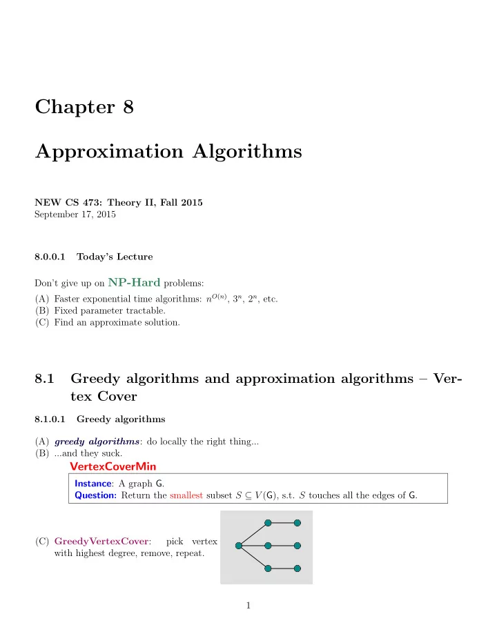
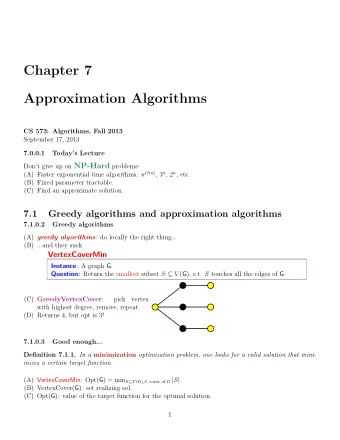
Chapter 8 Approximation Algorithms NEW CS 473: Theory II, Fall 2015 September 17, 2015 8.0.0.1 Today’s Lecture Don’t give up on NP-Hard problems: (A) Faster exponential time algorithms: n O ( n ) , 3 n , 2 n , etc. (B) Fixed parameter tractable. (C) Find an approximate solution. 8.1 Greedy algorithms and approximation algorithms – Ver- tex Cover 8.1.0.1 Greedy algorithms (A) greedy algorithms : do locally the right thing... (B) ...and they suck. VertexCoverMin Instance : A graph G . Question : Return the smallest subset S ⊆ V ( G ), s.t. S touches all the edges of G . (C) GreedyVertexCover : pick vertex with highest degree, remove, repeat. 1

8.1.1 Greedy algorithms 8.1.1.1 GreedyVertexCover in action... Observation 8.1.1. GreedyVertexCover returns 4 vertices, but opt is 3 vertices. 8.1.1.2 Good enough... Definition 8.1.2. In a minimization optimization problem, one looks for a valid solution that minimizes a certain target function. (A) VertexCoverMin : Opt( G ) = min S ⊆ V ( G ) ,S cover of G | S | . (B) VertexCover( G ): set realizing sol. (C) Opt( G ): value of the target function for the optimal solution. Definition 8.1.3. Alg is α -approximation algorithm for problem Min , achieving an approximation α ≥ 1, if for all inputs G , we have: Alg ( G ) Opt( G ) ≤ α. 8.1.1.3 Back to GreedyVertexCover (A) GreedyVertexCover : pick vertex with highest degree, remove, repeat. (B) Returns 4, but opt is 3! 2

(C) Can not be better than a 4 / 3-approximation algorithm. (D) Actually it is much worse! 8.1.1.4 How bad is GreedyVertexCover? Build a bipartite graph. Let the top partite set be of size n . In the bottom set add ⌊ n/ 2 ⌋ vertices of degree 2, such that each edge goes to a different vertex above. Repeatedly add ⌊ n/i ⌋ bottom vertices echo of degree i , for i = 2 , . . . , n . Repeatedly add ⌊ n/i ⌋ bottom vertices of degree i , for i = 2 , . . . , n . Repeatedly add ⌊ n/i ⌋ bottom vertices of degree i , for i = 2 , . . . , n . Repeatedly add ⌊ n/i ⌋ bottom vertices of degree i , for i = 2 , . . . , n . Bottom row has � n i =2 ⌊ n/i ⌋ = Θ( n log n ) vertices. 8.1.1.5 How bad is GreedyVertexCover? (A) Bottom row taken by Greedy. (B) Top row was a smaller solution. Lemma 8.1.4. The algorithm GreedyVertex- Cover is Ω(log n ) approximation to the optimal solution to VertexCoverMin . See notes for details! 3

8.1.2 How bad is GreedyVertexCover? 8.1.2.1 Understanding the graph... (A) Top row has n vertices. (B) Bottom row has (A) Upper bound: α = � n i =2 ⌊ n/i ⌋ ≤ � n i =1 n/i ≤ nH n = O ( n log n ) . (B) Lower bound: α = � n i =2 ⌊ n/i ⌋ ≥ � n i =1 n/i − ( n − 1) − n ≥ n ( H n − 2) ≥ n (ln n − 2) . (C) Bottom row has Θ( n log n ) vertices. (C) Greedy algorithm returns bottom row Θ( n log n ) vertices. (D) Optimal solution is top row: n vertices. (E) Greedy algorithm is O (log n ) approximation in this case. 8.1.2.2 Some math required � n n 1 1 � H n = i ≤ 1 + xdx = 1 + ln n − ln 1 = 1 + ln n. x =1 i =1 � �� � � i +1 1 / ( i +1) ≤ x = i (1 /x ) dx � n +1 n 1 1 � i ≥ = ln( n + 1 − ln 1 = ln( n + 1) H n = xdx x =1 i =1 � �� � � i +1 1 1 i ≥ x dx x = i ≥ ln n. Lemma 8.1.5. For H n = � n i =1 1 /i we have that ln n ≤ H n ≤ 1 + ln n . 8.1.2.3 Greedy Vertex Cover Theorem 8.1.6. The greedy algorithm for VertexCover achieves Θ(log n ) approximation, where n (resp. m ) is the number of vertices (resp., edges) in the graph. Running time is O ( mn 2 ) . Proof Lower bound follows from lemma. Upper bound follows from analysis of greedy algorithm for Set Cover , which will be done shortly. As for the running time, each iteration of the algorithm takes O ( mn ) time, and there are at most n iterations. 8.1.3 A better greedy algorithm: Two for the price of one 8.1.3.1 Two for the price of one - example 4

8.1.3.2 Two for the price of one ApproxVertexCover ( G ): S ← ∅ while E ( G ) � = ∅ do uv ← any edge of G S ← S ∪ { u, v } Remove u, v from V ( G ) Remove all edges involving u or v from E ( G ) return S Theorem 8.1.7. ApproxVertexCover is a 2 -approximation algorithm for VertexCoverMin that runs in O ( n 2 ) time. 8.2 Fixed parameter tractability, approximation, and fast ex- ponential time algorithms (to say nothing of the dog) 8.2.1 A silly brute force algorithm for vertex cover 8.2.1.1 What if the vertex cover is small? (A) G = ( V , E ) with n vertices (B) K ← Approximate VertexCoverMin up to a factor of two. (C) Any vertex cover of G is of size ≥ K/ 2. � n K +2 � (D) Naively compute optimal in O time. 8.2.1.2 Neighborhood of a vertex Definition 8.2.1. N G ( v ): Neighborhood of v – set of vertices of G adjacent to v . v N G ( v ) 5

8.2.1.3 Induced subgraph Definition 8.2.2. Let G = ( V , E ) be a graph. For a subset S ⊆ V , let G S be the induced subgraph over S . 8.2.2 Fixed parameter algorithm 8.2.2.1 Exact algorithm for Set Cover (A) G : Input graph. (B) Opt = min size vertex cover for G . opt = | Opt | . (C) Compute a set S ⊆ V ( G ) s.t. | S | ≤ 2 opt . Takes: O ( n + m ) time. (D) Enumerate over all possible X ⊆ S : (A) Check if X is vertex cover in G . Takes O ( n + m ) time. (E) Return smallest VC encountered. (F) Running time: O (2 2 opt ( n + m ) + n + m ) = O (2 2 opt m ). 8.2.2.2 Summary of result Theorem 8.2.3. Given a graph G with n vertices and m ( ≥ n ) edges, and with a vertex cover of size k . Then, one can compute the optimal vertex cover in G in O (2 2 k m ) time. Note, that running time is Fixed Parameter Tractable . 8.3 Traveling Salesperson Problem 8.3.0.1 TSP TSP-Min Instance : G = ( V, E ) a complete graph, and ω ( e ) a cost function on edges of G . Question : The cheapest tour that visits all the vertices of G exactly once. ≈ Solved exactly naively in n ! time. Using DP, solvable in O ( n 2 2 n ) time. 6

8.3.0.2 TSP Hardness Theorem 8.3.1. TSP-Min can not be approximated within any factor unless NP = P . Proof. (A) Reduction from Hamiltonian Cycle into TSP . (B) G = ( V , E ): instance of Hamiltonian cycle. (C) J : Complete graph over V . � 1 uv ∈ E ∀ u, v ∈ V w J ( uv ) = 2 otherwise . (D) ∃ tour of price n in J ⇐ ⇒ ∃ Hamiltonian cycle in G . (E) No Hamiltonian cycle = ⇒ TSP price at least n + 1. (F) But... replace 2 by cn , for c an arbitrary number 8.3.0.3 TSP Hardness - proof continued Proof: (A) Price of all tours are either: (i) n (only if ∃ Hamiltonian cycle in G ), (ii) larger than cn + 1 (actually, ≥ cn + ( n − 1)). (B) Suppose you had a poly time c -approximation to TSP-Min . (C) Run it on J : (i) If returned value ≥ cn + 1 = ⇒ no Ham Cycle since ( cn + 1) /c > n (ii) If returned value ≤ cn = ⇒ Ham Cycle since OPT ≤ cn < cn + 1 poly-time algorithm for NP-Complete problem. (D) c -approximation algorithm to TSP = ⇒ Possible only if P = NP . 8.3.1 TSP with the triangle inequality 8.3.1.1 Because it is not that bad after all. TSP △� = -Min Instance : G = ( V, E ) is a complete graph. There is also a cost function ω ( · ) defined over the edges of G , that complies with the triangle inequality. Question : The cheapest tour that visits all the vertices of G exactly once. triangle inequality : ω ( · ) if ∀ u, v, w ∈ V ( G ) , ω ( u, v ) ≤ ω ( u, w ) + ω ( w, v ) . Shortcutting σ : a path from s to t in G = ⇒ ω ( st ) ≤ ω ( σ ). 8.3.2 TSP with the triangle inequality 8.3.2.1 Continued... Definition 8.3.2. Cycle in G is Eulerian if it visits every edge of G exactly once. Assume you already seen the following: Lemma 8.3.3. A graph G has a cycle that visits every edge of G exactly once (i.e., an Eulerian cycle) if and only if G is connected, and all the vertices have even degree. Such a cycle can be computed in O ( n + m ) time, where n and m are the number of vertices and edges of G , respectively. 7

8.3.3 TSP with the triangle inequality 8.3.3.1 Continued... (A) C opt optimal TSP tour in G . � � (B) Observation : ω ( C opt ) ≥ weight cheapest spanning graph of G . (C) MST : cheapest spanning graph of G . ω ( C opt ) ≥ ω (MST( G )) � n � (D) O ( n log n + m ) = O ( n 2 ): time to compute MST . n = | V ( G ) | , m = . 2 8.3.4 TSP with the triangle inequality 8.3.4.1 2 -approximation (A) T ← MST ( G ) (B) J ← duplicate very edge of T . (C) H has an Eulerian tour. (D) C : Eulerian cycle in H . (E) ω ( C ) = ω ( H ) = 2 ω ( T ) = 2 ω ( MST ( G )) ≤ 2 ω ( C opt ). (F) π : Shortcut C so visit every vertex once. (G) ω ( π ) ≤ ω ( C ) 8.3.5 TSP with the triangle inequality 8.3.5.1 2 -approximation algorithm in figures s u s u D C v C v w w (a) (b) (c) (d) Euler Tour: vuvwvsv First occurrences: vuvwvsv Shortcut String: vuwsv 8.3.6 TSP with the triangle inequality 8.3.6.1 2 -approximation - result Theorem 8.3.4. G : Instance of TSP △� = -Min . C opt : min cost TSP tour of G . = ⇒ Compute a tour of G of length ≤ 2 ω ( C opt ) . 8