Social Network No introduc+on required Really? We - PowerPoint PPT Presentation
Mining Social Network Graphs Debapriyo Majumdar Data Mining Fall 2014 Indian Statistical Institute Kolkata November 13, 17, 2014 Social Network No introduc+on required Really? We s7ll
Mining ¡Social ¡Network ¡Graphs ¡ Debapriyo Majumdar Data Mining – Fall 2014 Indian Statistical Institute Kolkata November 13, 17, 2014
Social ¡Network ¡ No ¡introduc+on ¡required ¡ ¡ Really? ¡ ¡ We ¡s7ll ¡need ¡to ¡understand ¡a ¡ few ¡proper7es ¡ disclaimer: ¡the ¡brand ¡logos ¡are ¡used ¡here ¡en7rely ¡for ¡educa7onal ¡purpose ¡ ¡ 2 ¡
Social ¡Network ¡ § A collection of entities – Typically people, but could be something else too § At least one relationship between entities of the network – For example: friends – Sometimes boolean : two people are either friends or they are not – May have a degree – Discrete degree: friends, family, acquaintances, or none – Degree – real number : the fraction of the average day that two people spend talking to each other § An assumption of nonrandomness or locality – Hard to formalize – Intuition: that relationships tend to cluster – If entity A is related to both B and C, then the probability that B and C are related is higher than average (random) 3 ¡
Social ¡Network ¡as ¡a ¡Graph ¡ A B D E A graph with boolean (friends) C G F relationship § Check for the non-randomness criterion § In a random graph ( V,E ) of 7 nodes and 9 edges, if XY is an edge, YZ is an edge, what is the probability that XZ is an edge? – For a large random graph, it would be close to | E |/( | V | C 2 ) = 9/21 ~ 0.43 – Small graph: XY and YZ are already edges, so compute within the rest – So the probability is (| E| − 2)/( | V | C 2 − 2) = 7/19 = 0.37 § Now let’s compute what is the probability for this graph in particular Example ¡courtesy: ¡Leskovec, ¡Rajaraman ¡and ¡Ullman ¡ 4 ¡
Social ¡Network ¡as ¡a ¡Graph ¡ A B D E Does have A graph with boolean (friends) locality C G F relationship property § For each X , check possible YZ and check if YZ is an edge or not § Example: if X = A, YZ = {BC}, it is an edge X= YZ= Yes/Total X= YZ= Yes/Total A BC 1/1 E DF 1/1 B AC, AD, CD 1/3 F DE,DG,EG 2/3 C AB 1/1 G DF 1/1 BE,BG,BF,EF, D 2/6 Total 9/16 ~ 0.56 EG,FG 5 ¡
Types ¡of ¡Social ¡(or ¡Professional) ¡Networks ¡ A B D E C G F § Of course, the “social network”. But also several other types § Telephone network § Nodes are phone numbers § AB is an edge if A and B talked over phone within the last one week, or month, or ever § Edges could be weighted by the number of times phone calls were made, or total time of conversation 6 ¡
Types ¡of ¡Social ¡(or ¡Professional) ¡Networks ¡ A B D E C G F § Email network: nodes are email addresses § AB is an edge if A and B sent mails to each other within the last one week, or month, or ever – One directional edges would allow spammers to have edges § Edges could be weighted § Other networks: collaboration network – authors of papers, jointly written papers or not § Also networks exhibiting locality property 7 ¡
Clustering ¡of ¡Social ¡Network ¡Graphs ¡ § Locality property à there are clusters § Clusters are communities – People of the same institute, or company – People in a photography club – Set of people with “Something in common” between them § Need to define a distance between points (nodes) § In graphs with weighted edges, different distances exist § For graphs with “friends” or “not friends” relationship – Distance is 0 (friends) or 1 (not friends) – Or 1 (friends) and infinity (not friends) – Both of these violate the triangle inequality – Fix triangle inequality: distance = 1 (friends) and 1.5 or 2 (not friends) or length of shortest path 8 ¡
Tradi7onal ¡Clustering ¡ A B D E C G F § Intuitively, two communities § Traditional clustering depends on the distance – Likely to put two nodes with small distance in the same cluster – Social network graphs would have cross-community edges – Severe merging of communities likely § May join B and D (and hence the two communities) with not so low probability 9 ¡
Betweenness ¡of ¡an ¡Edge ¡ A B D E C G F § Betweenness of an edge AB: #of pairs of nodes (X,Y) such that AB lies on the shortest path between X and Y – There can be more than one shortest paths between X and Y – Credit AB the fraction of those paths which include the edge AB § High score of betweenness means? – The edge runs “between” two communities § Betweenness gives a better measure – Edges such as BD get a higher score than edges such as AB § Not a distance measure, may not satisfy triangle inequality. Doesn’t matter! 10 ¡
The ¡Girvan ¡– ¡Newman ¡Algorithm ¡ Calculate ¡ betweenness ¡of ¡edges ¡ § Step 1 – BFS: Start at a node X , perform a BFS with X as root 1 ¡ E § Observe: level of node Y = length 1 ¡ 1 ¡ of shortest path from X to Y D F § Edges between level are called Level ¡1 ¡ “DAG” edges – Each DAG edge is part of at B G least one shortest path from X Level ¡2 ¡ 1 ¡ 2 ¡ § Step 2 – Labeling: Label each node Y by the number of shortest paths from X to Y C A Level ¡3 ¡ 1 ¡ 1 ¡ 11 ¡
The ¡Girvan ¡– ¡Newman ¡Algorithm ¡ Calculate ¡betweenness ¡of ¡edges ¡ Step 3 – credit sharing: § Each leaf node gets credit 1 1 ¡ E § Each non-leaf node gets 1 + sum(credits of the DAG edges to the 4.5 ¡ 1 ¡ 1.5 ¡ level below) 1 ¡ D F § Credit of DAG edges: Let Y i ( i= 1, 4.5 ¡ Level ¡1 ¡ 1.5 ¡ … , k ) be parents of Z, p i = label( Y i ) 0.5 ¡ credit ( Y i , Z ) = credit ( Z ) × p i 3 ¡ 0.5 ¡ ( p 1 + ! p k ) B G Level ¡2 ¡ 1 ¡ § Intuition: a DAG edge Y i Z gets the 2 ¡ 3 ¡ share of credit of Z proportional to 1 ¡ the #of shortest paths from X to Z 1 ¡ 1 ¡ going through Y i Z Finally: Repeat Steps 1, 2 and 3 with C A Level ¡3 ¡ each node as root. For each edge, 1 ¡ 1 ¡ betweenness = sum credits obtained in all 1 ¡ 1 ¡ iterations / 2 12 ¡
Computa7on ¡in ¡prac7ce ¡ § Complexity: n nodes, e edges – BFS starting at each node: O ( e ) – Do it for n nodes – Total: O ( ne ) time – Very expensive § Method in practice – Choose a random subset W of the nodes – Compute credit of each edge starting at each node in W – Sum and compute betweenness – A reasonable approximation 13 ¡
Finding ¡Communi7es ¡using ¡Betweenness ¡ Method 1: § Keep adding edges (among existing ones) starting from lowest betweenness § Gradually join small components to build large connected components 14 ¡
Finding ¡Communi7es ¡using ¡Betweenness ¡ Method 1: § Keep adding edges (among existing ones) starting from lowest betweenness § Gradually join small components to build large connected components 15 ¡
Finding ¡Communi7es ¡using ¡Betweenness ¡ Method 1: § Keep adding edges (among existing ones) starting from lowest betweenness § Gradually join small components to build large connected components 16 ¡
Finding ¡Communi7es ¡using ¡Betweenness ¡ Method 1: § Keep adding edges (among existing ones) starting from lowest betweenness § Gradually join small components to build large connected components 17 ¡
Finding ¡Communi7es ¡using ¡Betweenness ¡ Method 1: § Keep adding edges (among existing ones) starting from lowest betweenness § Gradually join small components to build large connected components 18 ¡
Finding ¡Communi7es ¡using ¡Betweenness ¡ Method 1: § Keep adding edges (among existing ones) starting from lowest betweenness § Gradually join small components to build large connected components 19 ¡
Finding ¡Communi7es ¡using ¡Betweenness ¡ Method 2: § Start from all existing edges. The graph may look like one big component. § Keep removing edges starting from highest betweenness § Gradually split large components to arrive at communities 20 ¡
Finding ¡Communi7es ¡using ¡Betweenness ¡ Method 2: § Start from all existing edges. The graph may look like one big component. § Keep removing edges starting from highest betweenness § Gradually split large components to arrive at communities 21 ¡
Finding ¡Communi7es ¡using ¡Betweenness ¡ Method 2: § Start from all existing edges. The graph may look like one big component. § Keep removing edges starting from highest betweenness § Gradually split large components to arrive at communities At ¡some ¡point, ¡removing ¡the ¡edge ¡with ¡highest ¡betweenness ¡would ¡split ¡ the ¡graph ¡into ¡separate ¡components ¡ 22 ¡
Finding ¡Communi7es ¡using ¡Betweenness ¡ § For a fixed threshold of betweenness, both methods would ultimately produce the same clustering § However, a suitable threshold is not known beforehand § Method 1 vs Method 2 – Method 2 is likely to take less number of operations. Why? – Inter-community edges are less than intra-community edges 23 ¡
Recommend
More recommend
Explore More Topics
Stay informed with curated content and fresh updates.










![Tri rials Amit Garg [2,3,4,5] November 2020 Affiliations : [1] Department of Family Medicine,](https://c.sambuz.com/1037699/tri-rials-s.webp)
