Chapter 18 Learning from Examples 1 to lay out his tennis things - PDF document

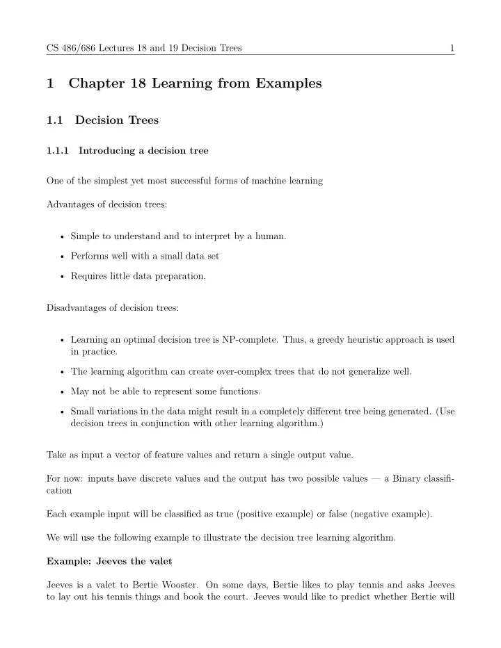
CS 486/686 Lectures 18 and 19 Decision Trees in practice. Jeeves is a valet to Bertie Wooster. On some days, Bertie likes to play tennis and asks Jeeves Example: Jeeves the valet We will use the following example to illustrate the decision tree learning algorithm. Each example input will be classifjed as true (positive example) or false (negative example). cation For now: inputs have discrete values and the output has two possible values — a Binary classifj- Take as input a vector of feature values and return a single output value. decision trees in conjunction with other learning algorithm.) • Small variations in the data might result in a completely difgerent tree being generated. (Use • May not be able to represent some functions. • The learning algorithm can create over-complex trees that do not generalize well. • Learning an optimal decision tree is NP-complete. Thus, a greedy heuristic approach is used 1 Disadvantages of decision trees: • Requires little data preparation. • Performs well with a small data set • Simple to understand and to interpret by a human. Advantages of decision trees: One of the simplest yet most successful forms of machine learning Introducing a decision tree 1.1.1 Decision Trees 1.1 Chapter 18 Learning from Examples 1 to lay out his tennis things and book the court. Jeeves would like to predict whether Bertie will

CS 486/686 Lectures 18 and 19 Decision Trees Overcast No 4 Overcast Hot High Strong Yes 5 Cool High Normal Weak Yes 6 Rain Hot High Weak Yes Strong Cool Overcast Mild Jeeves the valet – the test set Day Outlook Temp Humidity Wind Tennis? 1 Sunny High Rain Strong No 2 Rain Hot Normal Strong No 3 7 Mild Strong Sunny Weak Yes 12 Sunny Mild Normal Weak Yes 13 Cool Mild High Strong No 14 Sunny Cool High Weak No High Overcast Normal Rain Weak Yes 8 Overcast Cool High Weak Yes 9 Cool 11 High Weak Yes 10 Rain Mild Normal Strong No No High 2 High Overcast Hot High Weak Yes 4 Rain Mild Weak No Yes 5 Rain Cool Normal Weak Yes 6 Rain 3 Strong Normal Wind play tennis (and so be a better valet). Each morning over the last two weeks, Jeeves has recorded whether Bertie played tennis on that day and various attributes of the weather. Jeeves would like to evaluate the classifjer he has come up with for predicting whether Bertie will play tennis. Each morning over the next two weeks, Jeeves records the following data. Jeeves the valet – the training set Day Outlook Temp Humidity Tennis? High 1 Sunny Hot High Weak No 2 Sunny Hot Cool Strong Mild High 11 Sunny Mild Normal Strong Yes 12 Overcast Mild Strong Weak Yes 13 Overcast Hot Normal Weak Yes 14 Rain Yes Normal No High 7 Overcast Cool Normal Strong Yes 8 Sunny Mild Weak Mild No 9 Sunny Cool Normal Weak Yes 10 Rain A decision tree performs a sequence of tests in the input features.

CS 486/686 Lectures 18 and 19 Decision Trees 3 • Each node performs a test on one input feature. • Each arc is labeled with a value of the feature. • Each leaf node specifjes an output value. Using the Jeeves training set, we will construct two decision trees using difgerent orders of testing the features.

CS 486/686 Lectures 18 and 19 Decision Trees 4 The second and more complicated tree performs worse on the test examples than the fjrst tree, Yes. 10. Yes. 11. Yes. 12. No. 13. Yes. 14. Yes.) tree on the test examples. (1. Yes. 2. No. 3. No. 4. No. 5. Yes. 6. Yes/No. 7. Yes. 8. Yes. 9. The second tree classifjes 7/14 test examples correctly. Here are the decisions given by the second Yes. 9. Yes. 10. No. 11. Yes. 12. Yes. 13. No. 14. No. ) by the fjrst tree on the test examples. (1. No. 2. No. 3. No. 4. Yes. 5. Yes. 6. Yes. 7. Yes. 8. The fjrst (and simpler) tree classifjes 14/14 test examples correctly. Here are the decisions given One way to choose between the two is to evaluate them on the test set. Which tree would you prefer? We have constructed two decision trees and both trees can classify the training examples perfectly. will result in a really complicated tree shown on the next page. Example 2: Let’s construct another decision tree by choosing Temp as the root node. This choice Sunny No Outlook Example 1: Let’s construct a decision tree using the following order of testing features. Test Outlook fjrst. For Outlook=Sunny, test Humidity. (After testing Outlook, we could test any of the three re- maining features: Humidity, Wind, and Temp. We chose Humidity here.) For Outlook=Rain, test Wind. (After testing Outlook, we could test any of the three remaining features: Humidity, Wind, and Temp. We chose Wind here.) Humidity Yes Yes No Yes Wind possibly because the second tree is overfjtting to the training examples. Overcast Rain Weak Strong Normal High

CS 486/686 Lectures 18 and 19 Decision Trees R S O R W S M S W S O N No H W S H W N H S O R C Yes/No 5 Yes Temp Outlook Yes Yes Wind Yes No Outlook Wind No Yes Yes Humidity Yes Wind Yes No Wind Humidity Yes Outlook No S

CS 486/686 Lectures 18 and 19 Decision Trees 6 • The most important feature makes the most difgerence to the classifjcation of an example. • Solve the subproblems recursively. • Test the most important feature fjrst. • A greedy divide-and-conquer approach The decision-tree-learning algorithm: Use heuristics to fjnd a small consistent tree. Want a tree that is consistent with the examples and is as small as possible. Constructing a decision tree 1.1.2 How do we fjnd a good hypothesis in such a large space? truth tables. assume that every feature is binary.) For example, our simpler decision tree corresponds to the propositional formula. Every decision tree corresponds to a propositional formula. We hope to minimize the number of tests to create a shallow tree. ( Outlook = Sunny ∧ Humidity = Normal ) ∨ ( Outlook = Overcast ) ∨ ( Outlook = Rain ∧ Wind = Weak ) If we have n features, how many difgerent functions can we encode with decisions trees? (Let’s Each function corresponds to a truth table. Each truth table has 2 n rows. There are 2 2 n possible With n = 10 , 2 1024 ≈ 10 308 Intractable to fjnd the smallest consistent tree. (Intractable to search through 2 2 10 function.

CS 486/686 Lectures 18 and 19 Decision Trees Hot Sunny Hot High Weak Yes 3 Sunny Hot High Weak Yes 4 Sunny High No Weak Yes These four data points all have the same feature values, but the decisions are difgerent. This may happen if the decision is infmuenced by another feature that we don’t observe. For example, the decision may be infmuenced by Bertie’s mood when he woke up that morning, but Jeeves does not observe Bertie’s mood directly. • In this case, we return the majority decision of all the examples (breaking ties at random). When would we encounter the base case “no examples left”? • We encounter this base case when a certain combination of feature values does not appear in the training set. For example, the combination Temp = High, Wind = Weak, Humidity = High and Outlook = Rain does not appear in our training set. • In this case, we will choose the majority decision among all the examples in the parent node 2 Weak 7 end for The ID3 algorithm: Algorithm 1 ID3 Algorithm (Features, Examples 1: If all examples are positive, return a leaf node with decision yes. 2: If all examples are negative, return a leaf node with decision no. 3: If no features left, return a leaf node with the most common decision of the examples. 4: If no examples left, return a leaf node with the most common decision of the examples in the parent. 5: else 6: 7: 8: 9: High 10: When would we encounter the base case “no features left”? Temp Hot Sunny 1 Tennis? Wind Humidity Outlook • We encounter this case when the data is noisy and there are multiple difgerent decisions for Day • See the following example. the same set of feature values. (breaking ties at random). choose the most important feature f for each value v of feature f do add arc with label v add subtree ID 3( F − f, s ∈ S | f ( s ) = v )