Reinforcement learning Chapter 21, Sections 14 Chapter 21, Sections - PowerPoint PPT Presentation
Reinforcement learning Chapter 21, Sections 14 Chapter 21, Sections 14 1 Outline Examples Learning a value function for a fixed policy temporal difference learning Q-learning Function approximation Exploration
Reinforcement learning Chapter 21, Sections 1–4 Chapter 21, Sections 1–4 1
Outline ♦ Examples ♦ Learning a value function for a fixed policy – temporal difference learning ♦ Q-learning ♦ Function approximation ♦ Exploration Chapter 21, Sections 1–4 2
Reinforcement learning Agent is in an MDP or POMDP environment Only feedback for learning is percept + reward Agent must learn a policy in some form: – transition model T ( s, a, s ′ ) plus value function U ( s ) – Q ( a, s ) = expected utility if we do a in s and then act optimally – policy π ( s ) Chapter 21, Sections 1–4 3
Example: 4 × 3 world 3 + 1 2 − 1 1 START 1 2 3 4 (1 , 1) -.04 → (1 , 2) -.04 → (1 , 3) -.04 → (1 , 2) -.04 → (1 , 3) -.04 → · · · (4 , 3) +1 (1 , 1) -.04 → (1 , 2) -.04 → (1 , 3) -.04 → (2 , 3) -.04 → (3 , 3) -.04 → · · · (4 , 3) +1 (1 , 1) -.04 → (2 , 1) -.04 → (3 , 1) -.04 → (3 , 2) -.04 → (4 , 2) -1 . Chapter 21, Sections 1–4 4
Example: Backgammon 5 0 1 2 3 4 6 7 8 9 10 11 12 25 24 23 22 21 20 19 18 17 16 15 14 13 Reward for win/loss only in terminal states, otherwise zero TDGammon learns ˆ U ( s ) , represented as 3-layer neural network Combined with depth 2 or 3 search, one of top three players in world Chapter 21, Sections 1–4 5
Example: Animal learning RL studied experimentally for more than 60 years in psychology Rewards: food, pain, hunger, recreational pharmaceuticals, etc. Example: bees learn near-optimal foraging plan in field of artificial flowers with controlled nectar supplies Bees have a direct neural connection from nectar intake measurement to motor planning area Chapter 21, Sections 1–4 6
Example: Autonomous helicopter Reward = – squared deviation from desired state Chapter 21, Sections 1–4 7
Example: Autonomous helicopter Chapter 21, Sections 1–4 8
Temporal difference learning Fix a policy π , execute it, learn U π ( s ) Bellman equation: U π ( s ) = R ( s ) + γ s ′ T ( s, π ( s ) , s ′ ) U π ( s ′ ) � TD update adjusts utility estimate to agree with Bellman equation: U π ( s ) ← U π ( s ) + α ( R ( s ) + γ U π ( s ′ ) − U π ( s )) Essentially using sampling from the environment instead of exact summation Chapter 21, Sections 1–4 9
TD performance 0.6 1 (4,3) (3,3) 0.5 (1,3) 0.8 RMS error in utility 0.4 Utility estimates (1,1) (2,1) 0.6 0.3 0.4 0.2 0.2 0.1 0 0 0 100 200 300 400 500 0 20 40 60 80 100 Number of trials Number of trials Chapter 21, Sections 1–4 10
Q-learning One drawback of learning U ( s ) : still need T ( s, a, s ′ ) to make decisions Q ( a, s ) = expected utility if we do a in s and then act optimally Bellman equation: s ′ T ( s, π ( s ) , s ′ ) max a ′ Q ( a ′ , s ′ ) Q ( a, s ) = R ( s ) + γ � Q-learning update: a ′ Q ( a ′ , s ′ ) − Q ( a, s )) Q ( a, s ) ← Q ( a, s ) + α ( R ( s ) + γ max Q-learning is a model-free method for learning and decision making Q-learning is a model-free method for learning and decision making (so cannot use model to constrain Q-values, do mental simulation, etc.) Chapter 21, Sections 1–4 11
Function approximation For real problems, cannot represent U or Q as a table!! Typically use linear function approximation: ˆ U θ ( s ) = θ 1 f 1 ( s ) + θ 2 f 2 ( s ) + · · · + θ n f n ( s ) . Use a gradient step to modify θ parameters: U θ ( s )] ∂ ˆ U θ ( s ) θ i ← θ i + α [ R ( s ) + γ ˆ U θ ( s ′ ) − ˆ ∂θ i Q θ ( a, s )] ∂ ˆ Q θ ( a, s ) Q θ ( a ′ , s ′ ) − ˆ ˆ θ i ← θ i + α [ R ( s ) + γ max ∂θ i a ′ Often very effective in practice, but convergence not guaranteed Chapter 21, Sections 1–4 12
Exploration How should the agent behave? Choose action with highest expected utility? 3 +1 2 RMS error 1.5 Policy loss RMS error, policy loss 2 –1 1 0.5 1 0 0 50 100 150 200 250 300 350 400 450 500 1 2 3 4 Number of trials Exploration vs. exploitation : occasionally try “suboptimal” actions!! Chapter 21, Sections 1–4 13
Summary Reinforcement learning methods find approximate solutions to MDPs Work directly from experience in the environment Need not be given transition model a priori Q-learning is completely model-free Function approximation (e.g., linear combination of features) helps RL scale up to very large MDPs Exploration is required for convergence to optimal solutions Chapter 21, Sections 1–4 14
Recommend
More recommend
Explore More Topics
Stay informed with curated content and fresh updates.
