Learning from Data: Decision Trees Amos Storkey, School of - PowerPoint PPT Presentation

Learning from Data: Decision Trees Amos Storkey, School of Informatics University of Edinburgh Semester 1, 2004 LfD 2004

Decision Tree Learning - Overview • Decision tree representation • ID3 learning algorithm • Entropy, Information gain • Priors for Decision Tree Learning • Overfitting and how to avoid it • Reading: Mitchell, chapter 3 Acknowledgement: These slides are based on slides modified by Chris Williams and produced by Tom Mitchell, available from http://www.cs.cmu.edu/˜tom/ LfD 2004 1

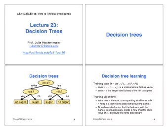
Decision trees • Decision tree learning is a method for approximating discrete-valued 1 target functions, in which the learned function is represented as a decision tree • Decision tree representation: – Each internal node tests an attribute – Each branch corresponds to attribute value – Each leaf node assigns a classification • Re-representation as if-then rules: disjunction of conjunctions of constraints on the attribute value instances 1 The method can be extended to learning continuous-valued functions LfD 2004 2

Decision Tree for Play Tennis Outlook Sunny Overcast Rain Wind Humidity Yes High Normal Strong Weak No Yes No Yes Logical Formulation: ( Outlook = Sunny ∧ Humidity = Normal ) ∨ ( Outlook = Overcast ) ∨ ( Outlook = Rain ∧ Wind = Weak ) LfD 2004 3

When to Consider Decision Trees • Instances describable by attribute–value pairs • Target function is discrete valued • Disjunctive hypothesis may be required • Possibly noisy training data Examples: • Equipment or medical diagnosis • Credit risk analysis • Modelling calendar scheduling preferences LfD 2004 4

Top-Down Induction of Decision Trees (ID3) 1. A is the “best” decision attribute for next node 2. Assign A as decision attribute for node 3. For each value of A , create new descendant of node 4. Sort training examples to leaf nodes 5. If training examples perfectly classified, Then STOP , Else iterate over new leaf nodes LfD 2004 5

Which attribute is best? A1=? A2=? [29+,35-] [29+,35-] t f t f [21+,5-] [8+,30-] [18+,33-] [11+,2-] LfD 2004 6

Entropy • S is a sample of training examples • p ⊕ is the proportion of positive examples in S • p ⊖ is the proportion of negative examples in S • Entropy measures the impurity of S Entropy ( S ) ≡ H ( S ) ≡ − p ⊕ log 2 p ⊕ − p ⊖ log 2 p ⊖ • H ( S ) = 0 if sample is pure (all + or all -), H ( S ) = 1 bit if p ⊕ = p ⊖ = 0 . 5 LfD 2004 7

Information Gain • Gain ( S, A ) = expected reduction in entropy due to sorting on A | S v | � Gain ( S, A ) ≡ Entropy ( S ) − | S | Entropy ( S v ) v ∈ V alues ( A ) • Information gain is also called the mutual information between A and the labels of S A1=? A2=? [29+,35-] [29+,35-] t f t f [21+,5-] [8+,30-] [18+,33-] [11+,2-] LfD 2004 8

Training Examples Day Outlook Temperature Humidity Wind PlayTennis D1 Sunny Hot High Weak No D2 Sunny Hot High Strong No D3 Overcast Hot High Weak Yes D4 Rain Mild High Weak Yes D5 Rain Cool Normal Weak Yes D6 Rain Cool Normal Strong No D7 Overcast Cool Normal Strong Yes D8 Sunny Mild High Weak No D9 Sunny Cool Normal Weak Yes D10 Rain Mild Normal Weak Yes D11 Sunny Mild Normal Strong Yes D12 Overcast Mild High Strong Yes D13 Overcast Hot Normal Weak Yes D14 Rain Mild High Strong No LfD 2004 9

Building the Decision Tree LfD 2004 10

Hypothesis Space Search by ID3 • Hypothesis space is complete! – Target function surely in there... • Outputs a single hypothesis (which one?) • No back tracking – Local minima... • “Batch” rather than “on-line” learning – More robust to noisy data... • Implicit prior: approx “prefer shortest tree” LfD 2004 11

Implicit priors in ID3 • Searching space from simple to complex, starting with empty tree, guided by information gain heuristic • Preference for short trees, and for those with high information gain attributes near the root • Bias is a preference for some hypotheses, rather than a restriction of hypothesis space • Occam’s razor: prefer the shortest hypothesis that fits the data LfD 2004 12

Occam’s Razor • Why prefer short hypotheses? • Argument in favour: – Fewer short hypotheses than long hypotheses − a short hypothesis that fits data unlikely to be coincidence − a long hypothesis that fits data might be coincidence • Argument opposed: – There are many ways to define small sets of hypotheses (notion of coding length ( X ) = − log 2 P ( X ) , Minimum Description Length ...) – e.g., all trees with a prime number of nodes that use attributes beginning with “Z” – What’s so special about small sets based on size of hypothesis?? LfD 2004 13

Overfitting in Decision Trees • Consider adding noisy training example #15: Sunny, Hot, Normal, Strong, PlayTennis = No • What effect on earlier tree? Outlook Sunny Overcast Rain Wind Humidity Yes High Normal Strong Weak No Yes No Yes LfD 2004 14

Overfitting in Decision Tree Learning • Overfitting can occur with noisy training examples, and also when small numbers of examples are associated with leaf nodes ( → coincidental or accidental regularities) 0.9 0.85 0.8 0.75 Accuracy 0.7 0.65 0.6 On training data On test data 0.55 0.5 0 10 20 30 40 50 60 70 80 90 100 Size of tree (number of nodes) LfD 2004 15

Avoiding Overfitting • How can we avoid overfitting? – stop growing when data split not statistically significant – grow full tree, then post-prune • How to select “best” tree: – Measure performance over training data – Measure performance over separate validation data set – MDL: minimize size ( tree ) + size ( misclassifications ( tree )) LfD 2004 16

Reduced-Error Pruning • Split data into training and validation set • Do until further pruning is harmful: 1. Evaluate impact on validation set of pruning each possible node (plus those below it) 2. Greedily remove the one that most improves validation set accuracy • produces smallest version of most accurate subtree • What if data is limited? LfD 2004 17

Effect of Reduced-Error Pruning 0.9 0.85 0.8 0.75 Accuracy 0.7 0.65 0.6 On training data On test data On test data (during pruning) 0.55 0.5 0 10 20 30 40 50 60 70 80 90 100 Size of tree (number of nodes) LfD 2004 18

Rule Post-Pruning 1. Convert tree to equivalent set of rules 2. Prune each rule independently of others, by removing any preconditions that result in improving its estimated accuracy 3. Sort final rules into desired sequence for use • Perhaps most frequently used method (e.g., C4.5) LfD 2004 19

Alternative Measures for Selecting Attributes • Problem: if an attribute has many values, Gain will select it • Example: use of dates in database entries • One approach: use GainRatio instead Gain ( S, A ) GainRatio ( S, A ) ≡ SplitInformation ( S, A ) c | S i | | S i | � SplitInformation ( S, A ) ≡ − | S | log 2 | S | i =1 where S i is subset of S for which A has value v i LfD 2004 20

Further points • Dealing with continuous-valued attributes—create a split, e.g. ( Temperature > 72 . 3) = t, f . Split point can be optimized (Mitchell, § 3.7.2) • Handling training examples with missing data (Mitchell, § 3.7.4) • Handling attributes with different costs (Mitchell, § 3.7.5) LfD 2004 21

Summary • Decision tree learning provides a practical method for concept learning/learning discrete-valued functions • ID3 algorithm grows decision trees from the root downwards, greedily selecting the next best attribute for each new decision branch • ID3 searches a complete hypothesis space, using a preference bias for smaller trees with higher information gain close to the root • The overfitting problem can be tackled using post-pruning LfD 2004 22