Brief Review of Probability Ken Kreutz-Delgado (Nuno Vasconcelos) - PowerPoint PPT Presentation
Brief Review of Probability Ken Kreutz-Delgado (Nuno Vasconcelos) ECE Department, UCSD ECE 175A - Winter 2012 Probability Probability theory is a mathematical language to deal with processes or experiments that are non-deterministic
Brief Review of Probability Ken Kreutz-Delgado (Nuno Vasconcelos) ECE Department, UCSD ECE 175A - Winter 2012
Probability • Probability theory is a mathematical language to deal with processes or experiments that are non-deterministic • Examples: – If I flip a coin 100 times, how many can I expect to see heads? – What is the weather going to be like tomorrow? – Are my stocks going to be up or down in value?
Sample Space = Universe of Outcomes • The most fundamental concept is that of a Sample Space (denoted by W or S or U ), also called the Universal Set . • A Random Experiment takes values in a set of Outcomes – The outcomes of the random experiment are used to define Random Events Event = Set of Possible Outcomes • Example of a Random Experiment : – Roll a single die twice consecutively – call the value on the up face at x 2 the n th toss x n for n = 1,2 6 – E.g., two possible experimental outcomes : two sixes ( x 1 = x 2 = 6 ) x 1 = 2 and x 2 = 6 • Example of a Random Event : 1 x 1 1 6 – An odd number occurs on the 2 nd toss .
Sample Space = Universal Event • The sample space U is a set of experimental outcomes that must satisfy the following two properties: – Collectively Exhaustive : all possible experimental outcomes are listed in the universal set U and when an experiment is performed one of these outcomes must occur . – Mutually Exclusive : only one outcomes happens and no other can occur (if x 1 = 5 it cannot be anything else). • The mutually exclusive property of outcomes simplifies the calculation of the probability of events • Collectively Exhaustive means that there is no possible event to which we cannot assign a probability • The Universe U (= sample space) of possible experimental outcomes is equal to the event “ Something Happens ” when an experiment is performed. Thus we also call U the Universal Event
Probability Measure • Probability of an event : – A positive real number between 0 and 1 expressing the chance that the event will occur when a random experiment is performed. • A probability measure satisfies the . Three Kolmogorov Axioms : . – P(A) 0 for any event A (every event A is a subset of U ) – P( U ) = P (Universal Event) = 1 (because “ something must happen ”) – if A B = , then P(A U B) = P(A) + P(B) x 2 6 • e.g. – P ( { x 1 0} ) = 1 1 x 1 1 6 – P ( { x 1 even } U { x 1 odd } ) = P ( { x 1 even } ) + P ( { x 1 odd } )
Probability Measure • The last axiom of the three, when combined with the mutually exclusive property of the sample set, – allows us to easily assign probabilities to all possible events if the probabilities of atomic events , aka elementary events , are known • Back to our dice example: – Suppose that the probability of the elementary event consisting of any single outcome-pair, A = {(x 1 ,x 2 )}, is P( A ) = 1/36 – We can then compute the probabilities of all events, including compound events : P( x 2 odd ) = 18x1/36 = 1/2 P( U ) = 36x1/36 = 1 P( two sixes ) = 1/36 P( x 1 = 2 and x 2 = 6 ) = 1/36
Probability Measure • Note that there are many ways to decompose the universal event U (the “ultimate” compound event) into the disjoint union of simpler events: – E.g. if A = { x 2 odd} , B = { x 2 even } , then U = A U B – on the other hand U = {( 1,1 )} U {( 1,2 )} U {( 1,3 )} U … U {( 6,6 )} – The fact that the sample space is exhaustive and mutually exclusive, combined with the three probability measure (Kolmogorov) axioms makes the whole procedure of computing the probability of a compound event from the probabilities of simpler events consistent.
Random Variables • A random variable X – is a function that assigns a real value to each sample space outcome – we have already seen one such function: P X ({x 1 ,x 2 }) = 1/36 for all outcome-pairs (x 1 ,x 2 ) (viewing an outcome as an atomic event) • Most Precise Notation: – Specify both the random variable, X , and the value, x , that it takes in your probability statements. E.g., X ( u ) = x for any outcome u in U . – In a probability measure , specify the random variable as a subscript, P X (x) ,and the value x as the argument. For example P X (x) = P X (x 1 ,x 2 ) = 1/36 means Prob[ X = ( x 1 ,x 2 )] = 1/36 – Without such care, probability statements can be hopelessly confusing
Random Variables • Types of random variables: – discrete and continuous (and sometimes mixed ) – Terminology relates to what types of values the RV can take • If the RV can take only one of a finite or at most countable set of possibilities, we call it discrete. – If there are furthermore only a finite set of possibilities, the discrete RV is finite . For example, in the two-throws-of-a-die example, there are only (at most) 36 possible values that an RV can take: x 2 6 1 x 1 1 6
Random Variables • If an RV can take arbitrary values in a real interval we say that the random variable is continuous • E.g. consider the sample space of weather temperature – we know that it could be any number between -50 and 150 degrees Celsius – random variable T [ -50,150 ] – note that the extremes do not have to be very precise, we can just say that P(T < -45 o ) = 0 • Most probability notions apply equal well to discrete and continuous random variables
Discrete RV • For a discrete RV the probability assignments given by a probability mass function ( pmf ) – this can be thought of as a normalized histogram a – satisfies the following properties 0 ( ) 1 , P a a X ( ) 1 P a X a • Example of a discrete (and finite) random variable – X { 1,2,3, … , 20 } where X = i if the grade of student z on class is greater than 5 ( i - 1 ) and less than or equal to 5i – We see from the discrete distribution plot that P X ( 15 ) = a
Continuous RV • For a continuous RV the probability assignments are given by a probability density function ( pdf ) – this is a piecewise continuous function that satisfies the following properties 0 ( ) P a a X ( ) 1 P a da X • Example for a Gaussian random variable of mean m and variance s 2 m 2 1 ( ) a ( ) exp P a s s X 2 2 2
Discrete vs Continuous RVs • In general the math is the same, up to replacing summations by integrals • Note that pdf means “density of the probability”, – This is probability per unit “area” (e.g., length for a scalar rv). – The probability of a particular value X = t of a continuous RV X is always zero Nonzero probabilities arise as: Pr( ) ( ) t X t dt P t dt X b Pr( ) ( ) a X b P t dt X a – Note also that pdfs are not necessarily upper bounded e.g. Gaussian goes to Dirac delta function when variance goes to zero
Multiple Random Variables • Frequently we have deal with with multiple random variables aka random vectors – e.g. a doctor’s examination measures a collection of random variable values: x 1 : temperature x 2 : blood pressure x 3 : weight x 4 : cough … • We can summarize this as – a vector X = ( X 1 , … , X n ) T of n random variables P X ( x 1 , … , x n ) is the joint probability distribution
Marginalization P ( cold ) ? • An important notion for multiple random variables is marginalization – e.g. having a cold does not depend on blood pressure and weight – all that matters are fever and cough – that is, we only need to know P X1,X4 (a,b) • We marginalize with respect to a subset of variables – (in this case X 1 and X 4 ) – this is done by summing (or integrating) the others out ( , ) ( , , , ) P x x P x x x x , 1 4 , , , 1 2 3 4 X X X X X X 1 4 1 2 3 4 , x x 3 4 ( , ) ( , , , ) P x x P x x x x dx dx , 1 4 , , , 1 2 3 4 2 3 X X X X X X 1 4 1 2 3 4
Conditional Probability ( | ) ? P X sick cough | Y • Another very important notion: – So far, doctor has P X1,X4 (fever,cough) – Still does not allow a diagnosis – For this we need a new variable Y with two states Y { sick, not sick } – Doctor measures the fever and cough levels. These are now no longer unknowns, or even (in a sense) random quantities. – The question of interest is “what is the probability that patient is sick given the measured values of fever and cough?” • This is exactly the definition of conditional probability – E.g., what is the probability that “Y = sick” given observations “X 1 = 98” and “X 2 = high”? We write this probability as: ( | 98 , ) P sick high | 1 , Y X X 4
Joint versus Conditional Probability • Note the very important difference between conditional and joint probability • Joint probability corresponds to an hypothetical question about probability over all random variables – E.g., what is the probability that you will be sick and cough a lot? ( , ) ? P X sick cough , Y
Conditional Probability • Conditional probability means that you know the values of some variables , while the remaining variables are unknown . – E.g., this leads to the question: what is the probability that you are sick given that you cough a lot? ( | ) ? P X sick cough | Y – “given” is the key word here – conditional probability is very important because it allows us to structure our thinking – shows up again and again in design of intelligent systems
Recommend
More recommend
Explore More Topics
Stay informed with curated content and fresh updates.





![CS70: Jean Walrand: Lecture 34. Uniformly at Random in [ 0 , 1 ] . Uniformly at Random in [ 0 , 1 ]](https://c.sambuz.com/987571/cs70-jean-walrand-lecture-34-uniformly-at-random-in-0-1-s.webp)
