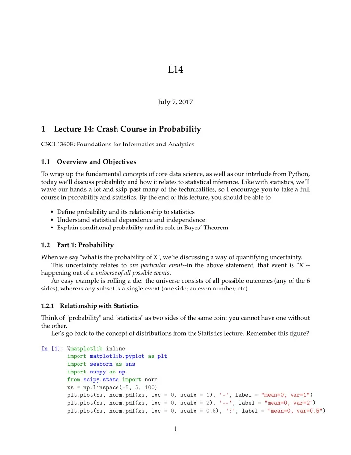

L14 July 7, 2017 1 Lecture 14: Crash Course in Probability CSCI 1360E: Foundations for Informatics and Analytics 1.1 Overview and Objectives To wrap up the fundamental concepts of core data science, as well as our interlude from Python, today we’ll discuss probability and how it relates to statistical inference. Like with statistics, we’ll wave our hands a lot and skip past many of the technicalities, so I encourage you to take a full course in probability and statistics. By the end of this lecture, you should be able to • Define probability and its relationship to statistics • Understand statistical dependence and independence • Explain conditional probability and its role in Bayes’ Theorem 1.2 Part 1: Probability When we say "what is the probability of X", we’re discussing a way of quantifying uncertainty. This uncertainty relates to one particular event --in the above statement, that event is "X"-- happening out of a universe of all possible events . An easy example is rolling a die: the universe consists of all possible outcomes (any of the 6 sides), whereas any subset is a single event (one side; an even number; etc). 1.2.1 Relationship with Statistics Think of "probability" and "statistics" as two sides of the same coin: you cannot have one without the other. Let’s go back to the concept of distributions from the Statistics lecture. Remember this figure? In [1]: %matplotlib inline import matplotlib.pyplot as plt import seaborn as sns import numpy as np from scipy.stats import norm xs = np.linspace(-5, 5, 100) plt.plot(xs, norm.pdf(xs, loc = 0, scale = 1), '-', label = "mean=0, var=1") plt.plot(xs, norm.pdf(xs, loc = 0, scale = 2), '--', label = "mean=0, var=2") plt.plot(xs, norm.pdf(xs, loc = 0, scale = 0.5), ':', label = "mean=0, var=0.5") 1
probstats plt.plot(xs, norm.pdf(xs, loc = -1, scale = 1), '-.', label = "mean=-1, var=1") plt.legend(loc = 0) plt.title("Various Normal Distributions") Out[1]: <matplotlib.text.Text at 0x11add7dd8> 2
These distributions allow us to say something about the probability of a random variable taking a certain specific value. In fact, if you look at the previous plot of the normal bell curves--picking a spot along one of those curves gives you the probability of the random variable representing that distribution taking on that particular value you picked! I hope it becomes clear that, the most likely value for a random variable to take is its mean. This even has a special name: the expected value . It means, on average, this is the value we’re going to get from this random variable. We have a special notation for probability: P ( X = x ) P is the universal symbol for "probability of", followed by some event . In this case, our event is " X = x ". (Recall from before: random variables are denoted with uppercase letters (e.g. X ), and observa- tions of that random variable are denoted with lowercase letters (e.g. x ). So when we say X = x , we’re asking for the event where the random variable takes on the value of the observation.) A few other properties to be aware of: • Probabilities are always between 0 and 1; no exceptions. This means, for any arbitrary event A , 0 ≤ P ( A ) ≤ 1. • The probability of something happening is always exactly 1. Put another way, if you combine all possible events together and ask the probability of one of them occurring, that probability is 1. 3
spinner • If A and B are two possible events that disparate (as in, they have no overlap), then the probability of either one of them happening is just the sum of their individual probabilities: P ( A , B ) = P ( A ) + P ( B ) . These three points are referred to as the Axioms of Probability and form the foundation for pretty much every other rule of probability that has ever been and will ever be discovered. 1.2.2 Visualizing A good way of learning probability is to visualize it. Take this spinner: It’s split into 12 segments. You could consider each segment to be one particular "event", and that event is true if, when you spin it, the spinner stops on that segment. So the probability of landing on any one specific segment is 1/12. The probability of landing on any segment at all is 1. 1.2.3 Dependence and Independence Two events A and B are dependent if having knowledge about one of them implicitly gives you knowledge about the other. On the other hand, they’re independent if knowing one tells you nothing about the other. Take an example of flipping a coin: I have a penny; a regular old penny. I flip it once, and it lands on Heads . I flip it 9 more times, and it lands on Heads each time. What is the probability that the next flip will be Heads ? 4
If you said 1/2, you’re correct! Coin flips are independent events; you could flip the coin 100 times and get 100 heads, and the probability of tails would still be 1/2. Knowing one coin flip or 100 coin flips tells you nothing about future coin flips. Now, I want to know what the probability is of two consecutive coin flips returning Heads. If the first flip is Heads, what is the probability of both flips being Heads? What if the first flip is Tails? In this case, the two coin flips are dependent . If the first flip is Tails, then it’s impossible for both coin flips to be Heads. On the other hand, if the first coin flip is Heads, then while it’s not certain that both coin flips can be Heads, it’s still a possibility. Thus, knowing one can tell you something about the other. If two events A and B are independent, their probability can be written as: P ( A , B ) = P ( A ) ∗ P ( B ) This is a huge simplification that comes up in many data science algorithms: if you can prove two random variables in your data are statistically independent, analyzing their behavior in con- cert with each other becomes much easier. On the other hand, if two events are dependent, then we can define the probabilities of these events in terms of their conditional probabilities : P ( A , B ) = P ( A | B ) ∗ P ( B ) This says "the probability of A and B is the conditional probability of A given B , multiplied by the probability of B ." 1.2.4 Conditional Probability Conditional probability is way of "fixing" a random variable(s) we don’t know, so that we can (in some sense) "solve" for the other random variable(s). So when we say: P ( A , B ) = P ( A | B ) ∗ P ( B ) This tells us that, for the sake of this computation, we’re assuming we know what B is in P ( A | B ) , as knowing B gives us additional information in figuring out what A is (again, since A and B are dependent). 1.2.5 Bayes’ Theorem Which brings us, at last, to Bayes’ Theorem and what is probably the hardest but most important part of this entire lecture. (Thank you , Rev. Thomas Bayes) Bayes’ Theorem is a clever rearrangement of conditional probability, which allows you to up- date conditional probabilities as more information comes in. For two events, A and B , Bayes’ Theorem states: P ( A | B ) = P ( B | A ) ∗ P ( A ) P ( B ) As we’ve seen, P ( A ) and P ( B ) are the probabilities of those two events independent of each other, P ( B | A ) is the probability of B given that we know A , and P ( A | B ) is the probability of A given that we know B . 1.2.6 Interpretation of Bayes’ Theorem Bayes’ Theorem allows for an interesting interpretation of probabilistic events. 5
bayes • P ( A | B ) is known as the posterior probability, which is the conditional event you’re trying to compute. • P ( A ) is known as the prior probability, which represents your current knowledge on the event A . • P ( B | A ) is known as the likelihood , essentially weighting how heavily the prior knowledge you have accumulated factors into the computation of your posterior. • P ( B ) is a normalizing factor--since the variable/event A , the thing we’re determining, is not involved in this quantity, it is essentially a constant. Given this interpretation, you could feasibly consider using Bayes’ Theorem as a procedure not only to conduct inference on some system, but to simultaneously update your understanding of the system by incorporating new knowledge. Here’s another version of the same thing (they use the terms "hypothesis" and "evidence", rather than "event" and "data"): 1.3 Review Questions Some questions to discuss and consider: 1: Go back to the spinner graphic. We know that the probability of landing on any specific segment is 1/12. What is the probability of landing on a blue segment? What about a red segment? What about a red OR yellow segment? What about a red AND yellow segment? 2: Recall the "conditional probability chain rule" from earlier in this lecture, i.e. that P ( A , B ) = P ( A | B ) ∗ P ( B ) . Given a coin with P ( heads ) = 0.75 and P ( tails ) = 0.25, and three coin flips A = heads , B = tails , C = heads , compute P ( A , B , C ) . 6
Recommend
More recommend