Polymers (continued) 18.S995 - L14 &15 dunkel@mit.edu - PowerPoint PPT Presentation

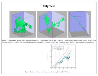
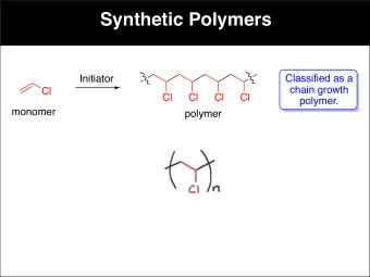
Polymers (continued) 18.S995 - L14 &15 dunkel@mit.edu

persistent RW model Karjalainen et al (2014) Polym Chem mechanistic model continuum model dunkel@math.mit.edu http://www.uni-leipzig.de/~pwm/web/?section=introduction&page=polymers

2.3 Continuum description 2.3.1 Di ff erential geometry of curves Consider a continuous curve r ( t ) ∈ R 3 , where t ∈ [0 , T ]. Assume that the first three r ( t ) , ... derivatives ˙ r ( t ) , ¨ r ( t ) are linearly independent. The length of the curve is given by Z T dt || ˙ L = r ( t ) || (2.41) 0 where ˙ r ( t ) = d r /dt and || · || denotes the Euclidean norm. The local unit tangent vector is defined by ˙ r t = r || . (2.42) || ˙ || || The unit normal vector, or unit curvature vector, is ( I − tt ) · ¨ r n = r || . (2.43) || ( I − tt ) · ¨ || · || − Unit tangent vector ˆ t ( t ) and unit normal vector ˆ n ( t ) span the osculating (‘kissing’) plane at point t . The unit binormal vector is defined by ( I − tt ) · ( I − nn ) · ... r b = r || . (2.44) || ( I − tt ) · ( I − nn ) · ... The orthonormal basis { t ( t ) , n ( t ) , b ( t ) } spans the local Frenet frame. For plane curves, ... r ( t ) is not linearly independent of ˙ r and ¨ r . In this case, we set b = t ∧ n . dunkel@math.mit.edu

- 2 ˙ r 0 t = || ˙ r || 2 2 0 - 2 2 ( I − tt ) · ¨ r n = || ( I − tt ) · ¨ r || 0 - 2 ( I − tt ) · ( I − nn ) · ... r b = || ( I − tt ) · ( I − nn ) · ... r || dunkel@math.mit.edu

∧ The local curvature κ ( t ) and the associated radius of curvature ρ ( t ) = 1 / κ are defined by ˙ t · n κ ( t ) = r || , (2.45) || ˙ || || and the local torsion τ ( t ) by τ ( t ) = ˙ n · b r || . (2.46) || ˙ For plane curves with constant b , we have τ = 0. Given || ˙ r || , κ ( t ), τ ( t ) and the initial values { t (0) , n (0) , b (0) } , the Frenet frames along the curve can be obtained by solving the Frenet-Serret system ˙ 0 1 0 1 0 1 t 0 0 t κ 1 A = A . ˙ n 0 (2.47a) n − κ τ @ @ A @ || ˙ r || ˙ 0 0 b b − τ The above formulas simplify if t is the arc length, for in this case || ˙ r || = 1. dunkel@math.mit.edu

2.3.2 Stretchable polymers: Minimal model and equipartition Z L � p E = γ 1 + h 2 (2.48) dx x � L , 0 where h x = h 0 ( x ). Restricting ourselves to small deformations, | h x | ⌧ 1, we may approxi- mate Z L E ' γ dx h 2 (2.49) x . 2 0 3 γ carries units of energy/length. dunkel@math.mit.edu

mate Z L E ' γ dx h 2 (2.49) x . 2 0 Taking into account that h (0) = h ( L ) = 0, we may represent h ( x ) and its derivative through the Fourier-sine series 1 ✓ n π x ◆ X h ( x ) = A n sin (2.50a) L n =1 X 1 ✓ n π x ◆ n π X h x ( x ) = A n L cos . (2.50b) L n =1 Exploiting orthogonality Z L ✓ n π x ◆ ✓ m π x ◆ = L dx sin sin (2.51) 2 δ nm L L 0 we may rewrite the energy (2.49) as Z L ✓ n π x ◆ ✓ m π x ◆ γ ⇣ n π ⌘ ⇣ m π ⌘ X X cos cos E dx A n A m ' 2 L L L L 0 n m ⌘ L γ ⇣ n π ⌘ ⇣ m π X X = A n A m 2 δ nm 2 L L n m 1 X = (2.52a) E n , n =1 where the energy E n stored in Fourier mode n is ✓ γ n 2 π 2 ◆ E n = A 2 (2.52b) . n 4 L dunkel@math.mit.edu

X X Z L 1 ✓ γ n 2 π 2 ◆ E ' γ X dx h 2 E n = A 2 = E n , x . n 2 4 L 0 n =1 Now assume the polymer is coupled to a bath and the stationary distribution is canonical 1 p ( { A n } ) = Z exp( � β E ) ∞  ✓ γ n 2 π 2 ◆� 1 X A 2 = Z exp � β (2.53) n 4 L X n =1 with β = ( k B T ) − 1 . The PDF factorizes and, therefore, also the normalization constant ∞ Y Z = Z n , (2.54a) i =1 where ✓ 4 π L ◆ 1 / 2 Z ∞ ✓ γ n 2 π 2  ◆� � β A 2 Z n = dA n exp = . (2.54b) n 4 L βγ n 2 π 2 ∞ dunkel@math.mit.edu

X X Z L 1 ✓ γ n 2 π 2 ◆ E ' γ X dx h 2 E n = A 2 = E n , x . n 2 4 L 0 n =1 Now assume the polymer is coupled to a bath and the stationary distribution is canonical 1 p ( { A n } ) = Z exp( � β E ) ∞  ✓ γ n 2 π 2 ◆� 1 X A 2 = Z exp � β (2.53) n 4 L  ✓ ◆� ✓ ◆ Z n =1 ∞ We thus find for the first to moments of A n E [ A n ] = 0 (2.55a) 2 k B TL E [ A 2 n ] = γ n 2 π 2 , (2.55b) and from this for the mean energy per mode ✓ γ n 2 π 2 ◆ n ] = 1 E [ A 2 E [ E n ] = 2 k B T. (2.56) 4 L dunkel@math.mit.edu

We may use the equipartition result to compute the variance of the polymer at the position x 2 [0 , L ] ∞ ∞ ✓ n π x ◆ ✓ m π x ◆ X X E [ h ( x ) 2 ] := E [ A n A m ] sin sin L L n =1 m =1 ∞ ∞ ✓ n π x ◆ ✓ m π x ◆ X X E [ A 2 = n ] δ nm sin sin L L n =1 m =1 sin 2 � � ∞ n π x/L ✓ 2 k B TL ◆ X = . (2.57) n 2 γπ 2 n =1 � � ✓ ◆ X If we additionally average along x ◆ π 2 ∞ ✓ k B TL ◆ ✓ k B TL 1 6 = k B TL X h E [ h ( x ) 2 ] i = n 2 = . (2.58) γπ 2 γπ 2 6 γ n =1 Thus, by measuring fluctuations along the polymer we may infer γ . dunkel@math.mit.edu

2.3.3 Rigid polymers: Euler-Bernoulli equation Z L E ' A dx κ 2 , (2.59) 2 0 where A is the bending modulus (units energy ⇥ length). For plane curves h ( x ), the curva- ture can be expressed as h xx κ = (2.60) x ) 3 / 2 . (1 + h 2 Focussing on the limit of weak deformations, h x ⌧ 1, we may approximate κ ' h xx , and the energy simplifies to Z L E ' A dx ( h xx ) 2 . (2.61) 2 0 dunkel@math.mit.edu

Boundary conditions Z L E ' A dx ( h xx ) 2 . (2.61) 2 0 The exact form of the boundary conditions depend on how the polymer is attached to the plane x = 0. Assuming that polymer is rigidly anchored at an angle 90 � , the boundary conditions at the fixed end at x = 0 are h (0) = 0 , h x (0) = 0 . (2.62a) At the free end, we will consider flux conditions h xx ( L ) = 0 , h xxx ( L ) = 0 . (2.62b) (minimal absolute curvature at the free end) dunkel@math.mit.edu

Boundary conditions Z L E ' A dx ( h xx ) 2 . (2.61) 2 0 By partial integrations, we may rewrite (2.61) as Z L " # L � A � E h x h xx dx h x h xxx ' � � 2 � 0 0 Z L  � A = dx h x h xxx � 2 0 Z L Z L " # L � � A = A � = � hh xxx + dx hh xxxx dx hh xxxx . (2.63) � 2 2 � 0 0 0 dunkel@math.mit.edu

If the polymer is surrounded by a viscous solvent, an initial perturbation h (0 , x ) will relax to the ground-state. Neglecting fluctuations due to thermal noise, the relaxation dynamics h ( t, x ) will be of the over-damped form 4 ⌘ h t = − � E � h , (2.64) where ⌘ is a damping constant, and the variational derivative is defined by � E [ h ( x )] E [ h ( x ) + ✏� ( x − y )] − E [ h ( x )] := lim . (2.65) � h ( y ) ✏ ✏ → 0 Keeping terms up to order ✏ , we find for the energy functional (2.61) Z L A dx [( h + ✏� ) xx ( h + ✏� ) xx − ( h xx ) 2 ] E [ h ( x ) + ✏� ( x − y )] − E [ h ( x )] = 2 0 Z L Z A dx [2 ✏ h xx � xx + O ( ✏ 2 )] = 2 0 Using the integral identity g ( x ) @ n x � ( x − y ) = ( − 1) n � ( x − y ) @ n x g ( x ) (2.66) for any smooth function g , one obtains Z L � E [ h ( x )] = A dx h xxxx ( x ) � ( x − y ) = Ah xxxx ( y ) , (2.67) � h ( y ) 0 dunkel@math.mit.edu

If the polymer is surrounded by a viscous solvent, an initial perturbation h (0 , x ) will relax to the ground-state. Neglecting fluctuations due to thermal noise, the relaxation dynamics h ( t, x ) will be of the over-damped form 4 ⌘ h t = − � E � h , (2.64) where ⌘ is a damping constant, and the variational derivative is defined by � E [ h ( x )] E [ h ( x ) + ✏� ( x − y )] − E [ h ( x )] := lim . (2.65) Z � h ( y ) ✏ ✏ → 0 so that Eq. (2.64) becomes a linear fourth-order equation ↵ = A h t = − ↵ h xxxx , ⌘ . (2.68) Inserting the ansatz h t = − 1 h = e − t/ ⌧ � ( x ) , ⌧ e − t/ ⌧ � , h xxxx = e − t/ ⌧ � xxxx , (2.69) gives the eigenvalue problem 1 ⌧↵� = � xxxx . (2.70) dunkel@math.mit.edu

Eigenvalue problem 1 ⌧↵� = � xxxx . (2.70) for the one-dimensional biharmonic operator ( @ 2 x ) 2 , which has the general solution � ( x ) = B 1 cosh( x/ � ) + B 2 sinh( x/ � ) + B 3 cos( x/ � ) + B 4 sin( x/ � ) (2.71a) where λ = ( ατ ) 1 / 4 . (2.71b) From the boundary conditions (2.62), we have 0 = B 1 + B 3 0 = B 2 + B 4 0 = B 1 cosh( L/ λ ) + B 2 sinh( L/ λ ) − B 3 cos( L/ λ ) − B 4 sin( L/ λ ) 0 = B 1 sinh( L/ λ ) + B 2 cosh( L/ λ ) + B 3 sin( L/ λ ) − B 4 cos( L/ λ ) dunkel@math.mit.edu

Inserting the first two conditions into the last two, we obtain the linear system 0 = B 1 [cosh( L/ λ ) + cos( L/ λ )] + B 2 [sinh( L/ λ ) + sin( L/ λ )] (2.73a) 0 = B 1 [sinh( L/ λ ) − sin( L/ λ )] + B 2 [cosh( L/ λ ) + cos( L/ λ )] . (2.73b) − For nontrivial solutions to exist, we must have ✓ [cosh( L/ λ ) + cos( L/ λ )] ◆ [sinh( L/ λ ) + sin( L/ λ )] 0 = det (2.74) [sinh( L/ λ ) − sin( L/ λ )] [cosh( L/ λ ) + cos( L/ λ )] which gives us the eigenvalue condition 0 = cosh( L/ λ ) cos( L/ λ ) + 1 . (2.75) This equation has solutions for discrete values λ n > 0 that can be computed numerically, and one finds for the first few eigenvalues L = { 0 . 94 , 2 . 35 , 3 . 93 , 5 . 50 , . . . } . (2.76) 2 λ n For comparison, for purely sinusoidal excitations of a harmonic string that L/ λ n ∝ n . dunkel@math.mit.edu