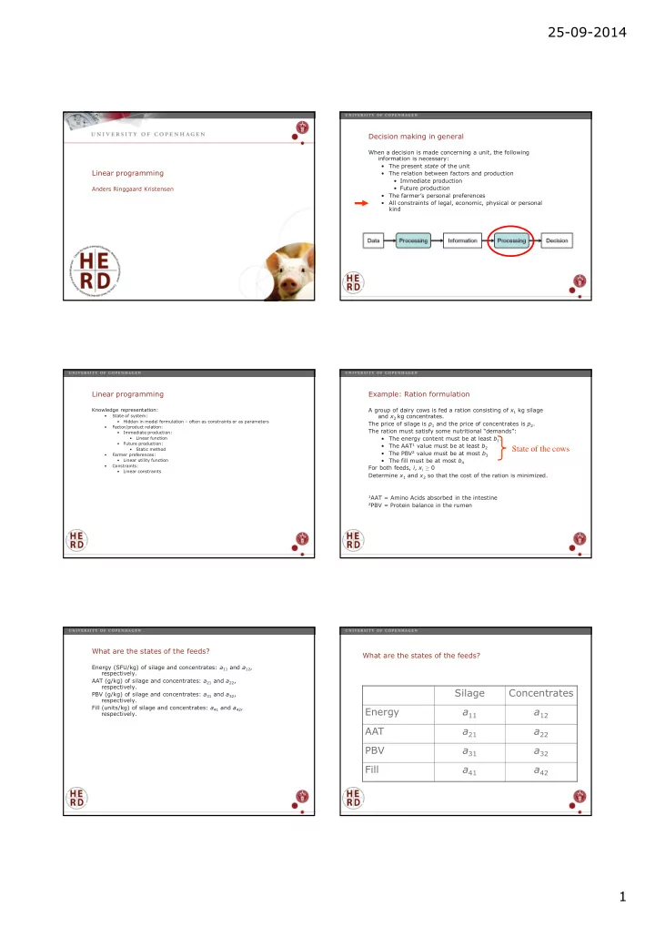
25-09-2014 Decision making in general When a decision is made - PDF document

25-09-2014 Decision making in general When a decision is made concerning a unit, the following information is necessary: • The present state of the unit Linear programming • The relation between factors and production • Immediate production • Future production Anders Ringgaard Kristensen • The farmer’s personal preferences • All constraints of legal, economic, physical or personal kind Linear programming Example: Ration formulation Knowledge representation: A group of dairy cows is fed a ration consisting of x 1 kg silage • State of system: and x 2 kg concentrates. • Hidden in model formulation – often as constraints or as parameters The price of silage is p 1 and the price of concentrates is p 2 . • Factor/product relation: The ration must satisfy some nutritional “demands”: • Immediate production: • The energy content must be at least b 1 . • Linear function The AAT 1 value must be at least b 2 • Future production: • State of the cows • Static method The PBV 2 value must be at most b 3 • • Farmer preferences: • The fill must be at most b 4 • Linear utility function • Constraints: For both feeds, i , x i ≥ 0 • Linear constraints Determine x 1 and x 2 so that the cost of the ration is minimized. 1 AAT = Amino Acids absorbed in the intestine 2 PBV = Protein balance in the rumen What are the states of the feeds? What are the states of the feeds? Energy (SFU/kg) of silage and concentrates: a 11 and a 12 , respectively. AAT (g/kg) of silage and concentrates: a 21 and a 22 , respectively. Silage Concentrates PBV (g/kg) of silage and concentrates: a 31 and a 32 , respectively. Fill (units/kg) of silage and concentrates: a 41 and a 42 , Energy a 11 a 12 respectively. AAT a 21 a 22 PBV a 31 a 32 Fill a 41 a 42 1

25-09-2014 LP problem LP - problem in matrix notation Objective function p 1 x 1 + p 2 x 2 = Min! (minimize costs) px = Min! - subject to - subject to a 11 x 1 + a 12 x 2 ≥ b 1 (energy at least b 1 ) Ax ≤ b a 21 x 1 + a 22 x 2 ≥ b 2 (AAT at least b 2 ) a 31 x 1 + a 32 x 2 ≤ b 3 (energy at most b 3 ) where p = ( p 1 , p 2 ), x = ( x 1 , x 2 )’, b = (- b 1 , - b 2 , b 3 , b 4 )’, and a 41 x 1 + a 42 x 2 ≤ b 4 (fill at most b 4 ) x 1 ≥ 0, x 2 ≥ 0 Constraints Graphical solution, convex area The linear relations: Two “activities” x 2 a 11 x 1 + a 12 x 2 ≥ b 1 ⇔ Energy, ≥ AAT, ≥ x 2 PBV, ≤ x 2 ≥ b 1 / a 12 – ( a 11 / a 12 ) x 1 Fill, ≤ The per-mitted area b 1 / a 12 forms a convex set The permitted area is bounded by a straight line in the diagram x 1 Slope: a 11 / a 12 x 1 The objective function Graphical solution, iso-cost line x 2 c’ / p 2 p 1 x 1 + p 2 x 2 = c (costs) For fixed cost c’ we have x 2 = c’ / p 2 – ( p 1 / p 2 ) x 1 Combinations of x 1 and x 2 having cost c’ Slope: p 1 / p 2 Combinations of x 1 and x 2 having same total cost form a straight line in the plane. We want to minimize cost c’ x 1 2

25-09-2014 Graphical solution, minimization What determines the optimum x 2 For a given set of constraints, the optimum is determined solely by the price relations. In our two-dimensional example it is simply the price ratio We want to minimize cost c’ p 1 / p 2 Decrease c’ until the permitted area is reached. Illustration Decrease c’ until the lowest value of the permitted area is found. Optimal combination is x 1 ’, x 2 ’ x 2 ’ x 1 x 1 ’ Influence of prices, I Influence of prices, II x 2 x 2 Original setting Slight increase of p 1 Drastic change in terms of x 1 and x 2 but only sligtly in terms of costs c x 2 ’ x 2 ’ x 1 x 1 x 1 ’ x 1 ’ Influence of prices, III Non-unique optimum x 2 x 2 Large increase of p 2 Increase of p 2 Drastic change in terms of x 1 and x 2 All combinations of x 1 and x 2 along a and to some extent c border are optimal x 2 ’ x 1 x 1 x 1 ’ 3

25-09-2014 Properties of linear programming Modeling tricks The permitted area is always a convex set The optimal solution is: From maximization to minimization: • Either uniquely located in a corner • p 1 x 1 + p 2 x 2 = Max! ⇔ - p 1 x 1 - p 2 x 2 = Min! • Or along a border line (accordingly also in two corners) From greater than to less than: It is therefore sufficient to search the corners of the convex set. • a i 1 x 1 + a i 2 x 2 ≥ b i ⇔ - a i 1 x 1 - a i 2 x 2 ≤ - b i From “equal to” to “less than” • a i 1 x 1 + a i 2 x 2 = b i ⇔ • - a i 1 x 1 - a i 2 x 2 ≤ - b i • a i 1 x 1 + a i 2 x 2 ≤ b i A convex set A non-convex set More than two variables The simplex algorithm The most commonly applied optimization algorithm for linear We cannot illustrate graphically anymore, but the same programming. principles apply: The simplex algorithm: • Convex (multi-dimensional) set • Identifies a corner of the convex set forming the permitted area. • Optimum always in a corner • Searches along the edges to find a better corner. • Checks whether the present corner is optimal Implemented in modern standard spreadsheets Implemented in ration formulation programs Shadow prices Basic assumptions of LP Proportionality What is the economic benefit of relaxing a constraint by one unit? • No start-up costs • No decreasing returns to scale • If it is not limiting it is zero! Additivity • Trivial method: • No interactions between activities Divisibility • Change the constraint by one • Any proportion of an activity allowed • Optimize again Certainty • How much did the result improve? • All parameters (coefficients, prices, constraints) are known precisely. • Software systems typically provides these values by default. 4

25-09-2014 McCull and his sheep & steers McCull: LP-problem McCull owns 200 ha of pasture where he can have ewes and/or Carrying capacity steers. Objective function: Gross margins are $24 per ewe and Season Ewes Steers 24 x 1 + 60 x 2 = Max! $60 per steer. Limited carrying capacity – refer to table Spring 15 5 Constraints: Summer 24 4 1/15 x 1 + 1/5 x 2 ≤ 200 Spring grazing 1/24 x 1 + 1/4 x 2 ≤ 200 Autumn 15 Summer grazing x 1 ≤ 3000 (i.e 15 x 200) Sheep in autumn Winter 8 x 1 ≤ 1600 (i.e 8 x 200) Sheep in winter x 1 ≥ 0, x 2 ≥ 0 McCull: Graphical solution Properties of methods for decision support Herd constraints Optimization 5000 Linear programming 4500 4000 3500 3000 2500 2000 Biological Functional 1500 variation limitations 1000 500 0 0 200 400 600 800 1000 Spring grazing Summer grazing Sheep in autumn Sheep in winter Iso-cost Uncertainty Dynamics 5