10.3 An Example of Postcontractual Hidden Knowledge: The Salesman - - PowerPoint PPT Presentation

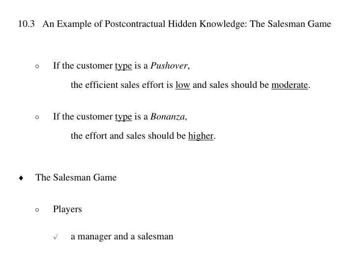
10.3 An Example of Postcontractual Hidden Knowledge: The Salesman Game

ð

If the customer is a , type Pushover the efficient sales effort is and sales should be . low moderate

ð

If the customer is a , type Bonanza the effort and sales should be . higher



The Salesman Game

ð

Players

r

a manager and a salesman

ð

The order of play 1 The

• ffers the salesman a
• f the form

manager contract [ ( ), ( )], w m q m where is the , is , and is a . w q m wage sales message 2 The salesman decides whether or not to accept the contract. 3 chooses whether the customer is a

• r

Nature type t Bonanza a with probabilities 0.2 and 0.8. Pushover The salesman the type, but the manager does .

• bserves

not

4 If the salesman has accepted the contract, he chooses his effort . e His sales level is , so his sales perfectly his effort. q e œ reveal 5 The salesman's is ( ) if he chooses ( ) wage w m e q m œ and zero otherwise.

ð

Payoffs

r

The manager is and the salesman is . risk-neutral risk-averse

r

If the salesman rejects the contract, his payoff is 8 and the manager's is zero. U _ œ

r

If he accepts the contract, then , and ( , , ), 1 1

manager salesman

œ  œ q w U e w t where 0, 0, 0, ` `  ` `  ` `  U e U e U w Î Î Î

2 2

and 0. ` ` 

2 2

U w Î

ð

The manager can perfectly effort, even out of equilibrium. deduce



The optimal contract

ð

The manager's indifference curves are with slope 1. straight lines

ð

The salesman's indifference curves slope , and are . upwards convex

r

The salesman has two sets of indifference curves, solid dashed for and for . Pushovers Bonanzas

ð

Figure 10.1

r

The truth-telling is the contract

• ptimal

contract pooling that pays the intermediate wage of w3 for the intermediate quantity of , and q3 zero for any other quantity, regardless of the . message

r

The pooling contract is a contract, second-best a between the optimum for and compromise Pushovers the optimum for . Bonanzas

r

The contract must satisfy the constraint, participation 0.8 ( , , ) 0.2 ( , , ) 8. U q w Pushover U q w Bonanza

3 3 3 3



ð

The

• f the equilibrium depends on the
• f the indifference

nature shapes curves.

ð

Figure 10.2

r

The equilibrium is , not pooling, and separating there does exist a , contract. first-best fully revealing

r

The contract induces the salesman to be , and truthful the constraints are satisfied. incentive compatibility

ð

The idea is to reward salesmen just for effort, not high but for effort. appropriate



Another way to look at a equilibrium is separating to think of it as a

• f contracts rather than

choice as contract with different for different .

• ne

wages

• utputs

ð

In this interpretation, the manager offers a

• f contracts and

menu the salesman selects

• f them
• ne

after type learning his .



The Salesman Game illustrates a number of . ideas

ð

It can have either a

• r a

equilibrium. pooling separating

ð

The can be applied to avoid revelation principle having to consider contracts in which the manager must interpret the salesman's . lies

ð

It shows how to use when the functions are diagrams algebraic intractable or unspecified.

10.4 The Groves Mechanism

ð

The principal is an government altruistic that cares directly about the utility of the agents.

r

a benevolent government

ð

The mayor is considering installing a costing $100. streetlight

r

He will only install it if he decides that the sum of the residents' valuations cost for it is greater than or equal to the .

r

The mayor's problem is to their valuations. discover



The Streetlight Game

ð

Players

r

the mayor and householders five

ð

The order of play Nature chooses the value vi that householder places on having a streetlight installed, i using ( ). distribution f v

i i

Only householder . i v

• bserves

i

1 The mayor announces a , , mechanism M which requires a householder who to ( ) reports pay m w m if the streetlight is installed, and installs the streetlight if ( ) 100 0. g m , m , m , m , m m

1 2 3 4 5 1 5

´  

j j œ

2 Householder reports value i m

i simultaneously

with all other householders. 3 If ( ) 0, g m , m , m , m , m

1 2 3 4 5

the streetlight is and householder pays ( ). built i w mi

ð

Payoffs

r

The mayor tries to maximize , social welfare including the welfare of besides the 5 . taxpayers householders

r

His payoff is zero if the streetlight is built. not

r

Otherwise, it is 1mayor

j j

100, œ  

œ1 5

v subject to the constraint that ( ) 100, 

j j œ1 5

w m so he can raise the taxes to pay for the light.

r

The payoff of householder is zero i if the streetlight is built. not

r

Otherwise, it is 1i

i i

( ) ( ). m , m , m , m , m v w m

1 2 3 4 5

œ 



Mechanisms

ð

Mechanism M1

r

   w m Build iff m ( ) 20, 100

i j j

œ

œ1 5

r

Talk is cheap, and the strategy would be to

• r

. dominant

• verreport

underreport

r

a mechanism flawed

ð

Mechanism M2

r

   w m Max m Build iff m ( ) { , 0}, 100

i i j j

œ

œ1 5

r

If all the householders each other's perfectly, knew values then there would be a

• f Nash equilibria

continuum that attained the result. efficient

r

Each householder would announce up to his valuation if necessary.

ð

Mechanism M3

r

    w m m Build iff m ( ) 100 , 100

i j j j i j

œ 

Á œ1 5

r

a Nash equilibrium in which all the players are truthful

r

a mechanism dominant-strategy

ñ

Truthfulness is weakly . dominant

ñ

The players are strictly better off telling the truth whenever would alter the mayor's . lying decision

r

It is budget-balancing. not

r

The total tax revenue could easily be . negative

10.5 Price Discrimination

ð

A problem of under adverse selection mechanism design



Varian's Nonlinear Pricing Game

ð

Players

r

• ne seller and one buyer

ð

The order of play

assigns the buyer a , . Nature type s The buyer is "unenthusiastic" with utility function or u "valuing" with utility function , with probability. v equal The seller does

• bserve Nature's move, but the buyer

. not does 1 The

• ffers

{ , } seller mechanism w q

m m

under which the can announce his as and buyer type m buy amount for lump sum . q w

m m

2 The chooses a

• r rejects the mechanism entirely

buyer message m and does not buy at all.

ð

Payoffs

r

The seller has a marginal cost, so his is . zero payoff w w

u v



r

The buyers' are ( ) and ( ) payoffs 1 1

u u u v v v

œ  œ  u q w v q w if is positive, and 0 if 0, q q œ with , 0 and , 0. u v u v

w w ww ww

 

r

The marginal willingness to pay is for the valuing buyer: greater for any , q u q v q

w w

( ) ( ). (10.27) 

ð

Condition (10.27) is an example of the property. single-crossing

r

Combined with the assumption that (0) (0) 0, v u œ œ it also implies that ( ) ( ) for any value of . u q v q q 

Perfect Price Discrimination

ð

The game would allow price discrimination perfect if the seller did which buyer had which utility function. know

ð

The seller's maximization problem

r

Maximize w w q q w w

u v u v u v

, , ,  subject to the constraints participation

ñ

u q w ( )

u u



ñ

v q w ( )

v v



ð

The constraints will be satisfied as . equalities

r

w u q

u u

œ ( )

r

w v q

v v

œ ( )

ð

The seller's maximization problem rewritten

r

Maximize u q v q q q

u v u v

, ( ) ( ) 

ð

u q v q

w w

( ) 0 ( )

* * u v

œ œ w u q w v q

* * * * u u v v

œ œ ( ) ( )

r

The consumer surpluses are eaten up. entire

Interbuyer Price Discrimination

ð

The price discrimination problem arises interbuyer when the seller knows which utility functions Smith and Jones have and can sell to them . separately

ð

Assume that the must charge each buyer a price per unit seller single and let the choose the quantity. buyer

ð

The seller's maximization problem

r

Maximize p q p q q q p p

u v u v u u v v

, , ,  subject to the constraints participation

ñ

u q p q ( )

u u u



ñ

v q p q ( )

v v v

 and the constraints incentive compatibility

ñ

q argmax u q p q

u u u u

œ [ ( ) ] 

ñ

q argmax v q p q

v v v v

œ [ ( ) ] 

ð

The buyers' problems quantity choice

r

u q p

w(

)

u u

 œ

r

v q p

w(

)

v v

 œ

ð

The seller's maximization problem rewritten

r

Maximize u q q v q q q q

u v u u v v

, ( ) ( )

w w

 subject to the constraints participation

ñ

u q u q q ( ) ( )

u u u



w

ñ

v q v q q ( ) ( )

v v v



w

ð

The participation constraints will be binding. not

r

u q u q q q ( ) ( ) is increasing in .

u u u u



w

r

v q v q q q ( ) ( ) is increasing in .

v v v v



w

ð

The first-order conditions

r

u q q u q

ww w

( ) ( )

u u u

 œ

r

v q q v q

ww w

( ) ( )

v v v

 œ

r

two problems independent

ð

If the function were a more general function ( ), cost convex c q q

u v

 the two first-order conditions would have to be solved , together because each condition would depend on both and . q q

u v

Back to Nonlinear Pricing

ð

Interquantity price discrimination

r

The seller charges different for different . unit prices quantities

ð

Neither nor the perfect price discrimination the interbuyer problems are mechanism design problems.

r

The seller is perfectly about the

• f the buyers.

informed types

ð

The original game is a problem of mechanism design under adverse selection.

r

Separation is the seller's main concern.

r

The seller designs incentives to separate the

• f the buyers.

types



The equilibrium mechanism

ð

The seller's maximization problem

r

Maximize w w q q w w

u v u v u v

, , ,  subject to the constraints participation

ñ

u q w ( )

u u



ñ

v q w ( )

v v

 and the constraints self-selection

ñ

u q w u q w ( ) ( )

u u v v

 

ñ

v q w v q w ( ) ( )

v v u u

 

ð

Not binding all of these constraints will be .

r

In a mechanism design problem like this, what always happens is that the are designed contracts so that type of agent is pushed down to his .

• ne

reservation utility

‰

Suppose that the optimal is in fact , and contract separating also that types accept a contract. both

‰

The consumer's constraint is . unenthusiastic participation binding

r

w u q

u u

œ ( )

‰

The consumer's constraint is . valuing self-selection binding

r

w w v q v q

v u u v

œ  ( ) ( ) 

ð

The seller's maximization problem reformulated Maximize u q u q v q v q q q

u v u u u v

, ( ) ( ) ( ) ( )   

ð

The first-order conditions

r

u q u q v q

w w w

( ) { ( ) ( )}

u u u

  œ

r

v q

w(

)

v

œ

‰

The type buys a such that his last unit's valuing quantity marginal utility exactly the marginal cost of production. equals

r

v q

w(

)

** v

œ

r

His consumption is at the level. efficient

‰

The type buys than his amount. unenthusiastic less first-best

r

the property that ( ) ( ) single-crossing u q v q

w w



r

u q u q v q

w w w

( ) { ( ) ( )}

u u u

  œ

r

u q

w(

)

** u



‰

The seller must sell than

• ptimal

less first-best to the type unenthusiastic so as not to make that too attractive to the type. contract valuing

‰

On the other hand, making the type's more valuable valuing contract to him actually helps , separation so is chosen to maximize . q

v

social surplus

‰

q q

** ** u v



r

the property that ( ) ( ) single-crossing u q v q

w w



r

v q

ww( )



r

u q v q

w w

( ) 0 and ( )

** ** u v

 œ

‰

The equilibrium is , not pooling. separating

‰

A corner solution

ð

Despite facing a monopolist, the type can end up retaining consumer surplus valuing  an . informational rent

r

a return to his information about his own type private

The Single-Crossing Property

‰

Condition (10.27) is an example of the property, single-crossing since it implies that the

• f the two agents

indifference curves cross at most time.

• ne

‰

The buyer has demand than the buyer. valuing stronger unenthusiastic

r

u q v q q

w w

( ) ( ) for all 

‰

Two curves satisfying the property single-crossing

r

u q q ( ) œ 

r

v q q ( ) 2 œ 

‰

It is often natural to assume that the property holds, and single-crossing it is a useful condition for to be possible, sufficient separation but it is a necessary condition. not