1 An Filtering System that Monitors Document Search Engines Can - PDF document
Filtering May be Your Work Adaptive Information Filtering Using Bayesian Graphical Models Yi Zhang Baskin School of Engineering University of California Santa Cruz yiz@soe.ucsc.edu 1 2 Filtering May be Your Work Filtering May be Your Work
Filtering May be Your Work Adaptive Information Filtering Using Bayesian Graphical Models Yi Zhang Baskin School of Engineering University of California Santa Cruz yiz@soe.ucsc.edu 1 2 Filtering May be Your Work Filtering May be Your Work Getting potential terrorist alert Tracking stock news 3 4 Filtering May be Your Work Even if You Do Not Work… Getting funding alerts 5 6 1
An Filtering System that Monitors Document Search Engines Can Help, But … Not Enough! Stream(s) • Search engine focus: Short term information need (ad free text initialization query hoc search) document stream – Information source is relatively static Delivered docs – User pulls information from the system … • The task: Long term information need (adaptive Filtering System J filtering) (binary classifier) – Information source is dynamic (user profile) – User wants to be alerted as soon as the information is available – System pushes information to the user learning accumulated Feedback docs user profile 7 8 Related Areas Common Approaches and Problems in IR Focus of • Many people work on filtering Applications Models this talk – More than 40+ institutes Events tracking – NIST TREC filtering track, SPAM track, TDT • Bioinformatics Commonly used evaluation measure: Utility Statistics, optimization – Example: T9U=2 J - L � deliver if P( J |document)>=0.33 Business applications Artificial Intelligence • Commonly used algorithms: relevance based filtering Information Medical informatics Machine learning – Relevance retrieval + Threshold Filtering Digital library – Binary text classification: relevant vs. non-relevant Natural language processing • Challenges and opportunities Email filtering – Very limited user supervision Human computer interaction … – User criteria beyond relevance Database – Complex user models can be learned over a long period of user interaction Computer networks – Poor performance with existing algorithms Computer systems Security Systems 9 10 Our Approach: What are Bayesian Graphical Models (BGM)? System with Desirable Characteristics Three Components What can a Our solution Unified person do? • Bayesian axiom: maximizing utility for a computer Framework (desirable characteristics) • Representation tools: Graphical Model – Graphical representation summarizes conditional independence Use heuristics Bayesian Prior relationships between variables on the graph – Conditional probabilistic distributions or potential functions Bayesian encode the quantitative relationship between connected nodes Bayesian Graphical • Inference algorithms Ask good Active Learning Models questions – Estimating the unknown from the known – Methods to achieve the goal of utility maximizing v0 Use multiple forms Graphical of evidence Models P(v1|v0) v1 v2 Bayesian Social learning Hierarchical 11 12 P(v3|v1,v2) v3 Modeling 2
Road Map Motivation: Using Heuristics as Bayesian Prior • Introduction priors • How we use BGM for filtering variance mean – Using expert’s heuristics as a Bayesian prior (SIGIR04) – Exploration and exploitation trade off using Bayesian active learning (ICML 03) document – Combining multiple forms of evidence using graphical models (HLT 05) parameter X P ( w | mean , var iance ) w – Collaborative adaptive user modeling with explicit & implicit feedback (CIKM 06) • Contribution and future work Y relevant = P ( y yes | x , w ) 13 14 Method: Convert Decision Boundary to Prior Distribution When is it Expected to Work? 1 = ∏ P ( w | D ) p ( y | x , w ) P ( w ) t i i Z ( D ) Rocchio + threshold => w R i t = P ( w ) N ( w | w , v ) m hypothesis: learner: low bias logistic regression w * performance T = ∏ heuristic algorithm w arg max p ( y | x , w ) m i i w * i = 1 w = α w used to estimate m R and cosine( w , w ) = 1 w R prior: low variance R Document space (N) Logistic Regression Parameter space (N+1) Rocchio algorithm •Step 1 : Heuristic algorithm => w R T = α * α * = ∏ α •Step 2: w w where arg max p ( y | x , w ) m R i i R α i = 1 •Step 3: Use w m as logistic regression prior mean number of training data 15 •Step 4: Estimate posterior distribution of logistic parameter 16 Results Road Map 0.8 our team: 0.6 our Logistic_Rocchio LR_Rocchio • Introduction Logistic Regression Team 1 normalized utility 0.7 Rocchio 0.5 • How we use BGM for filtering 0.6 Team 2 Logistic_UnscaledRocchio – Using expert’s heuristics as a Bayesian prior 0.4 0.5 Team 4 0.4 – Exploration and exploitation trade off using Bayesian active learning 0.3 0.3 – Combining multiple forms of evidence using graphical models 0.2 0.2 – Collaborative adaptive user modeling with explicit & implicit feedback 0.1 0.1 • Contribution and future work 0 0 TREC 11 Adaptive Filtering Data TDT 2004 results reported by NIST •Best TREC official result: 0.475 •A little better result (0.7328) reported by team_1 in the TDT workshop •Similar performance on TREC 9 data 17 18 3
Motivation: A “Bad” Document May Help Future Performance Exploitation: Estimate U immediate • The effects of delivering a document to the user: Using Bayesian Inference, we have: – A: Satisfy a user’s information need immediately – B: Get the user feedback, learn from it, and serve the user better � U ( d | D ) = U ( d | θ ) P ( θ | D ) d θ in the future immediate t t − 1 immediate t t − 1 • Existing filtering systems don’t consider the effect B or consider θ � it heuristically θ = θ U ( d | ) A P ( y | d , ) immediate t y t • Our solution: Bayesian active learning y – Model the future utility of delivering a document explicitly Y=relevant or non relevant while learning the threshold Ay : credit/penalty defined by the utility function = + U ( d ) U ( d ) N U ( d ) � � � � � immediate � future � � � future � � � d t : document arrives at current time t A : exploitati on B : exploratio n D t-1 : existing training data set before d t arrives 19 20 Method: Estimating Future Utility Using Bayesian Decision Theory The Whole Process on BGM ∧ • • Step 1: Estimate the immediate utility When the true model is , we incur some loss if using model θ θ model: θ P θ : ( | D ) ∧ ∧ ∧ t − 1 U ( d | D ) θ θ − Loss ( θ , θ ) = U ( θ , θ ) − U ( θ , θ ) immediate t t 1 � �������������� = θ θ θ U ( d | ) P ( | D ) d • immediate t t − 1 The true model is unknown, but given training data set D, we estimate the θ posterior distribution of the true model, and then estimate the expected loss of ∧ using : θ • Step 2: Estimate the future utility document: d t ∧ ∧ Loss ( θ ) = E Loss ( θ , θ ) P ( θ | D ) ( | ) U d D future t t − 1 � ∧ • Measure the quality of training data set D as the expected loss of using � θ = Loss ( D ) − P ( y | d , D ) Loss ( D ( d , y )) D t − 1 t t − 1 t − 1 t ^ = θ Loss ( D ) Loss ( ) y D relevant: y • Step 3: Deliver d t if and only if • Measure the future utility as the expected reduction on loss = − � U ( d ) = U ( d | D ) + N U ( d | D ) > 0 U ( d | D ) Loss ( D ) E Loss ( D ( d , y )) − − − t immediate t t − 1 future future t t − 1 future t t 1 t 1 P ( y | d , D ) t 1 t t t − 1 21 22 Results Road Map Trec-10: Reuters Dataset Trec-9: OHSUMED Dataset • Introduction • How we use BGM for filtering Bayesian Bayesian Bayesian Bayesian Active Immediate Active Immediate – Using expert’s heuristics as a Bayesian prior normalized 0.448 0.445 normalized 0.353 0.360 – Exploration and exploitation trade off using Bayesian active learning utility utility – Combining multiple forms of evidence using graphical models (beyond utility 3534 3149 utility 11.32 11.54 relevance) docs/profile 4527 3895 docs/profile 31 25 » User study » Data analysis • When exploration is worth doing, it is • When exploration is not worth doing, it – Collaborative adaptive user modeling with explicit & implicit feedback effective didn’t hurt • Contribution and future work – thousands of relevant documents – active learning didn’t improve – only 51 out of 300000 are relevant documents on average 23 24 4
Recommend
More recommend
Explore More Topics
Stay informed with curated content and fresh updates.
