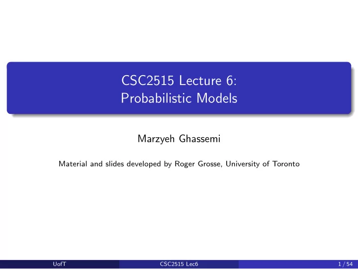
CSC2515 Lecture 6: Probabilistic Models Marzyeh Ghassemi Material - PowerPoint PPT Presentation

CSC2515 Lecture 6: Probabilistic Models Marzyeh Ghassemi Material and slides developed by Roger Grosse, University of Toronto UofT CSC2515 Lec6 1 / 54

Today’s Agenda Bayesian parameter estimation: average predictions over all hypotheses, proportional to their posterior probability. Generative classification: learn to model the distributions of inputs belonging to each class Na¨ ıve Bayes (discrete inputs) Gaussian Discriminant Analysis (continuous inputs) UofT CSC2515 Lec6 2 / 54

Data Sparsity Maximum likelihood has a pitfall: if you have too little data, it can overfit. E.g., what if you flip the coin twice and get H both times? UofT CSC2515 Lec6 3 / 54

Data Sparsity Maximum likelihood has a pitfall: if you have too little data, it can overfit. E.g., what if you flip the coin twice and get H both times? N H 2 θ ML = = 2 + 0 = 1 N H + N T Because it never observed T, it assigns this outcome probability 0. This problem is known as data sparsity. If you observe a single T in the test set, the log-likelihood is −∞ . UofT CSC2515 Lec6 3 / 54

Bayesian Parameter Estimation In maximum likelihood, the observations are treated as random variables, but the parameters are not. The Bayesian approach treats the parameters as random variables as well. UofT CSC2515 Lec6 4 / 54

Bayesian Parameter Estimation In maximum likelihood, the observations are treated as random variables, but the parameters are not. The Bayesian approach treats the parameters as random variables as well. To define a Bayesian model, we need to specify two distributions: The prior distribution p ( θ ), which encodes our beliefs about the parameters before we observe the data The likelihood p ( D | θ ), same as in maximum likelihood UofT CSC2515 Lec6 4 / 54

Bayesian Parameter Estimation In maximum likelihood, the observations are treated as random variables, but the parameters are not. The Bayesian approach treats the parameters as random variables as well. To define a Bayesian model, we need to specify two distributions: The prior distribution p ( θ ), which encodes our beliefs about the parameters before we observe the data The likelihood p ( D | θ ), same as in maximum likelihood When we update our beliefs based on the observations, we compute the posterior distribution using Bayes’ Rule: p ( θ ) p ( D | θ ) p ( θ | D ) = p ( θ ′ ) p ( D | θ ′ ) d θ ′ . � We rarely ever compute the denominator explicitly. UofT CSC2515 Lec6 4 / 54

Bayesian Parameter Estimation Let’s revisit the coin example. We already know the likelihood: L ( θ ) = p ( D ) = θ N H (1 − θ ) N T It remains to specify the prior p ( θ ). UofT CSC2515 Lec6 5 / 54

Bayesian Parameter Estimation Let’s revisit the coin example. We already know the likelihood: L ( θ ) = p ( D ) = θ N H (1 − θ ) N T It remains to specify the prior p ( θ ). We can choose an uninformative prior, which assumes as little as possible. A reasonable choice is the uniform prior. But our experience tells us 0.5 is more likely than 0.99. One particularly useful prior that lets us specify this is the beta distribution: p ( θ ; a , b ) = Γ( a + b ) Γ( a )Γ( b ) θ a − 1 (1 − θ ) b − 1 . This notation for proportionality lets us ignore the normalization constant: p ( θ ; a , b ) ∝ θ a − 1 (1 − θ ) b − 1 . UofT CSC2515 Lec6 5 / 54

Bayesian Parameter Estimation Beta distribution for various values of a , b : Some observations: The expectation E [ θ ] = a / ( a + b ). The distribution gets more peaked when a and b are large. The uniform distribution is the special case where a = b = 1. The main thing the beta distribution is used for is as a prior for the Bernoulli distribution. UofT CSC2515 Lec6 6 / 54

Bayesian Parameter Estimation Computing the posterior distribution: p ( θ | D ) ∝ p ( θ ) p ( D | θ ) � θ a − 1 (1 − θ ) b − 1 � � � θ N H (1 − θ ) N T ∝ = θ a − 1+ N H (1 − θ ) b − 1+ N T . This is just a beta distribution with parameters N H + a and N T + b . UofT CSC2515 Lec6 7 / 54

Bayesian Parameter Estimation Computing the posterior distribution: p ( θ | D ) ∝ p ( θ ) p ( D | θ ) � θ a − 1 (1 − θ ) b − 1 � � � θ N H (1 − θ ) N T ∝ = θ a − 1+ N H (1 − θ ) b − 1+ N T . This is just a beta distribution with parameters N H + a and N T + b . The posterior expectation of θ is: N H + a E [ θ | D ] = N H + N T + a + b UofT CSC2515 Lec6 7 / 54

Bayesian Parameter Estimation Computing the posterior distribution: p ( θ | D ) ∝ p ( θ ) p ( D | θ ) � θ a − 1 (1 − θ ) b − 1 � � � θ N H (1 − θ ) N T ∝ = θ a − 1+ N H (1 − θ ) b − 1+ N T . This is just a beta distribution with parameters N H + a and N T + b . The posterior expectation of θ is: N H + a E [ θ | D ] = N H + N T + a + b The parameters a and b of the prior can be thought of as pseudo-counts. The reason this works is that the prior and likelihood have the same functional form. This phenomenon is known as conjugacy, and it’s very useful. UofT CSC2515 Lec6 7 / 54

Bayesian Parameter Estimation Bayesian inference for the coin flip example: Small data setting N H = 2, N T = 0 UofT CSC2515 Lec6 8 / 54

Bayesian Parameter Estimation Bayesian inference for the coin flip example: Small data setting Large data setting N H = 2, N T = 0 N H = 55, N T = 45 When you have enough observations, the data overwhelm the prior. UofT CSC2515 Lec6 8 / 54

Bayesian Parameter Estimation What do we actually do with the posterior? The posterior predictive distribution is the distribution over future observables given the past observations. We compute this by marginalizing out the parameter(s): � p ( D ′ | D ) = p ( θ | D ) p ( D ′ | θ ) d θ . (1) UofT CSC2515 Lec6 9 / 54

Bayesian Parameter Estimation What do we actually do with the posterior? The posterior predictive distribution is the distribution over future observables given the past observations. We compute this by marginalizing out the parameter(s): � p ( D ′ | D ) = p ( θ | D ) p ( D ′ | θ ) d θ . (1) For the coin flip example: θ pred = Pr ( x ′ = H | D ) � p ( θ | D ) Pr ( x ′ = H | θ ) d θ = � = Beta ( θ ; N H + a , N T + b ) · θ d θ = E Beta ( θ ; N H + a , N T + b ) [ θ ] N H + a = (2) N H + N T + a + b , UofT CSC2515 Lec6 9 / 54

Bayesian Parameter Estimation Bayesian estimation of the mean temperature in Toronto Assume observations are i.i.d. Gaussian with known standard deviation σ and unknown mean µ Broad Gaussian prior over µ , centered at 0 We can compute the posterior and posterior predictive distributions analytically (full derivation in notes) Why is the posterior predictive distribution more spread out than the posterior distribution? UofT CSC2515 Lec6 10 / 54

Bayesian Parameter Estimation Comparison of maximum likelihood and Bayesian parameter estimation Some advantages of the Bayesian approach More robust to data sparsity Incorporate prior knowledge Smooth the predictions by averaging over plausible explanations UofT CSC2515 Lec6 11 / 54

Bayesian Parameter Estimation Comparison of maximum likelihood and Bayesian parameter estimation Some advantages of the Bayesian approach More robust to data sparsity Incorporate prior knowledge Smooth the predictions by averaging over plausible explanations Problem: maximum likelihood is an optimization problem, while Bayesian parameter estimation is an integration problem This means maximum likelihood is much easier in practice, since we can just do gradient descent Automatic differentiation packages make it really easy to compute gradients There aren’t any comparable black-box tools for Bayesian parameter estimation (although Stan can do quite a lot) UofT CSC2515 Lec6 11 / 54

Maximum A-Posteriori Estimation Maximum a-posteriori (MAP) estimation: find the most likely parameter settings under the posterior This converts the Bayesian parameter estimation problem into a maximization problem ˆ θ MAP = arg max p ( θ | D ) θ p ( θ ) p ( D | θ ) = arg max θ log p ( θ ) + log p ( D | θ ) = arg max θ UofT CSC2515 Lec6 12 / 54

Maximum A-Posteriori Estimation Joint probability in the coin flip example: log p ( θ, D ) = log p ( θ ) + log p ( D | θ ) = const + ( a − 1) log θ + ( b − 1) log(1 − θ ) + N H log θ + N T log(1 − θ ) = const + ( N H + a − 1) log θ + ( N T + b − 1) log(1 − θ ) UofT CSC2515 Lec6 13 / 54

Maximum A-Posteriori Estimation Joint probability in the coin flip example: log p ( θ, D ) = log p ( θ ) + log p ( D | θ ) = const + ( a − 1) log θ + ( b − 1) log(1 − θ ) + N H log θ + N T log(1 − θ ) = const + ( N H + a − 1) log θ + ( N T + b − 1) log(1 − θ ) Maximize by finding a critical point d θ log p ( θ, D ) = N H + a − 1 − N T + b − 1 0 = d 1 − θ θ UofT CSC2515 Lec6 13 / 54

Maximum A-Posteriori Estimation Joint probability in the coin flip example: log p ( θ, D ) = log p ( θ ) + log p ( D | θ ) = const + ( a − 1) log θ + ( b − 1) log(1 − θ ) + N H log θ + N T log(1 − θ ) = const + ( N H + a − 1) log θ + ( N T + b − 1) log(1 − θ ) Maximize by finding a critical point d θ log p ( θ, D ) = N H + a − 1 − N T + b − 1 0 = d 1 − θ θ Solving for θ , N H + a − 1 ˆ θ MAP = N H + N T + a + b − 2 UofT CSC2515 Lec6 13 / 54