Convergence of the Ensemble Kalman Filter Jan Mandel Center for - PowerPoint PPT Presentation

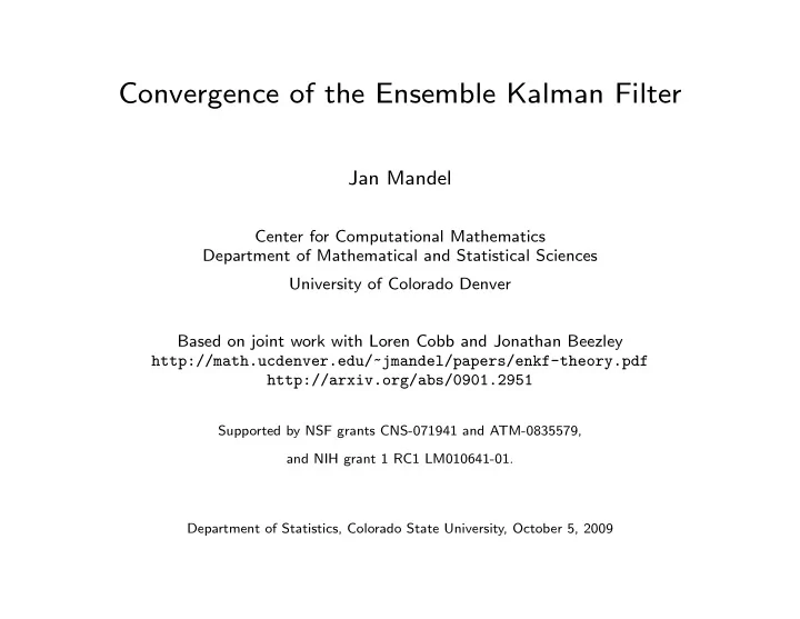
Convergence of the Ensemble Kalman Filter Jan Mandel Center for Computational Mathematics Department of Mathematical and Statistical Sciences University of Colorado Denver Based on joint work with Loren Cobb and Jonathan Beezley http://math.ucdenver.edu/~jmandel/papers/enkf-theory.pdf http://arxiv.org/abs/0901.2951 Supported by NSF grants CNS-071941 and ATM-0835579, and NIH grant 1 RC1 LM010641-01. Department of Statistics, Colorado State University, October 5, 2009

Data assimilation • Goal: Inject data into a running model • Approach: discrete time filtering = sequential statistical estimation • Model state is a random variable U with probability density p ( u ) • Data + measurement error enter as data likelihood p ( d | u ) • Probability densities updated by Bayes theorem : p ( u ) ∝ p ( d | u ) p f ( u ) Analysis cycle time k − 1 advance time k time k analysis model forecast analysis U ( k − 1) U ( k ) ,f U ( k ) Bayesian − → − → − → p ( k − 1) ( u ) p ( k − 1) ( u ) p ( k ) ( u ) update data ր likelihood p ( d | u )

Kalman filter • Model state U is represented by its mean and covariance. • Assume that the forecast is Gaussian, U f ∼ N ( m f , Q f ), and • the data likelihood is Gaussian, p ( d | u ) ∝ exp[ − ( Hu − d ) T R − 1 ( Hu − d ) / 2]. • Then the analysis is also Gaussian, U ∼ N ( m, Q ), given by m = m f + K ( d − Hm f ) , Q = ( I − KH ) Q f where K = Q f H T ( HQ f H T + R ) − 1 is the gain matrix • Hard to advance the covariance matrix when the model is nonlinear • Needs to maintain the covariance matrix - unsuitable for large problems • Ensemble Kalman filter (EnKF): represent U by an ensemble and estimate Cov U by the sample covariance.

Ensemble Kalman filter (EnKF) • represent model state by an ensemble,covariance → sample covariance • apply Kalman formulas for the mean to the ensemble members • perturb data to get the correct analysis ensemble covariance Algorithm 1. Generate initial i.i.d. ensemble X 1 , . . . , X N 2. In each analysis cycle Advance the model in time: forecast X f i = M ( X i ) Compute the sample covariance Q f N of the forecast ensemble Get randomized data: D i ∼ d + E i , i.i.d. E i ∼ N (0 , R ) Bayesian update: analysis X i = X f k + K N ( D i − HX f i ) where K N = Q f N H T ( HQ f N H T + R ) − 1

EnKF properties • The model is needed only as a black box. • The EnKF was derived for Gaussian distributions. • It is often used for nonlinear models and non-Gaussian distributions. • The EnKF was designed so that the ensemble is a sample from the correct analysis distribution if - the forecast ensemble is i.i.d. and Gaussian - the covariance matrix is exact • But - the sample covariance matrix is a random variable - the ensemble is not independent: sample covariance ties it together - the ensemble is not Gaussian: the update step is nonlinear

Convergence analysis overview • Goal: show that asymptotically, for large ensemble - the sample covariance converges to the exact covariance - the ensemble is asymptotically i.i.d. - the ensemble is asymptotically Gaussian - the ensemble members converge to the correct distribution • Roadmap: - the ensemble is exchangeable: plays the role of independent - the ensemble is a-priori bounded in L p : plays the role of Gaussian - use the weak law of large numbers for the sample covariance - the ensemble converges to a Gaussian i.i.d. ensemble obtained with the exact covariance matrix instead of the sample covariance - tools: weak convergence and L p convergence of random variables

Tools: Weak convergence Weak convergence of probability measures: µ n ⇒ µ � fdµ n → � fdµ ∀ continuous bounded f if Weak convergence of random elements: X n ⇒ X if law ( X n ) ⇒ law ( X ) Continuous mapping theorem: if X n ⇒ X and g is continuous, then g ( X n ) ⇒ g ( X ) Joint weak convergence: if X n ⇒ X and Y n ⇒ C (constant), then ( X n , Y n ) ⇒ ( X, C ) Slutsky’s theorem: if X n ⇒ X and Y n ⇒ C are random variables, then X n + Y n ⇒ X + C and X n Y n ⇒ XC

Tools: L p convergence Stochastic L p norm of a random element X : � X � p = ( E ( | X | p )) 1 /p L p convergence implies weak convergence: if X n → X in L p , then X n ⇒ X Uniform integrability: if X n ⇒ X and { X n } bounded in L p , then X n → X in L q ∀ q < p

Convergence to Kalman filter � � • Generate the initial ensemble X (0) X (0) N 1 , . . . , X (0) = i.i.d. and N NN Gaussian. � � X ( k ) N 1 , . . . , X ( k ) • Run EnKF, get ensembles . NN • For theoretical purposes, define U (0) = X (0) and U ( k ) by EnKF ex- N N N cept with the exact covariance of the filtering distribution instead of the sample covariance. • Then U ( k ) is a sample (i.i.d.) from the Gaussian filtering distribution N (as would be delivered by the Kalman filter). • We will show that X ( k ) Ni → U ( k ) Ni in L p for all p < ∞ as N → ∞ , for all analysis cycles k .

A-priori properties of EnKF ensembles Exchangeability Definition: set of r.v. is exchangeable if their joint distribution is per- mutation invariant. Lemma: All EnKF ensembles are exchangeable. Proof: The initial ensemble in EnKF is i.i.d., thus exchangeable, and the analysis step is permutation invariant.

A-priori properties of EnKF ensembles L p bounds Lemma. All EnKF ensembles are bounded in L p with constant indepen- dent of N , for all p < ∞ . Proof ingredients: • Recall that X ( k ) = X ( k ) ,f + K ( k ) N ( D ( k ) N − H ( k ) X ( k ) ,f ) N N N K ( k ) = Q ( k ) ,f H ( k ) T ( H ( k ) Q ( k ) ,f H ( k ) T + R ( k ) ) − 1 N N N • Bound � Q ( k ) ,f � p from the L 2 p bound on X ( k ) ,f N N • Bound the matrix norm | ( H ( k ) Q ( k ) ,f H ( k ) T + R ( k ) ) − 1 | ≤ const N from R ( k ) > 0 (positive definite).

Convergence of sample mean �� � � �� X N 1 X NN , . . . , are exchangeable, { U N 1 , . . . , U NN } Lemma. If U N 1 U NN are i.i.d., U N 1 ∈ L 2 is the same for all N , and X N 1 → U N 1 in L 2 , then X N = ( X N 1 + · · · + X NN ) /N ⇒ E ( U N 1 ) . Note that { U N 1 , . . . , U NN } and { X N 1 , . . . , X NN } are not independent. Proof ingredients: � � Exchangeability gives � X Ni − U Ni � 2 → 0 and Cov X Ni , X Nj → 0 independent of i , j . Standard Monte-Carlo argument: 2 = Var( X N ) � � � X N − E ( X N 1 ) � � � N N = 1 � � Var( X Ni ) + Cov( X Ni , X Nj ) N 2 i =1 i,j =1 ,j � = j = 1 N Var( X N 1 ) + (1 − 1 N ) Cov( X N 1 , X N 2 ) → 0

Convergence of sample covariance �� � � �� X N 1 X NN Lemma. If , . . . , are exchangeable, { U N 1 , . . . , U NN } U N 1 U NN are i.i.d., U N 1 ∈ L 4 is the same for all N , and X N 1 → U N 1 in L 4 , then the sample covariance of ( X N 1 , . . . , X NN ) ⇒ Cov ( U N 1 ) , N → ∞ . Proof ingredients: Entries of the sample covariance are [ X N X T N ] jℓ − [ X Ni ] j [ X Ni ] ℓ . L 4 bound on X Ni gives L 2 bound on the products [ X Ni ] j [ X Ni ] ℓ , thus the sample mean of the products converges. Use convergence of the sample mean X N and Slutsky’s theorem.

Recall EnKF ensemble and reference KF ensemble Initial ensemble X (0) N is Gaussian i.i.d., then generate X ( k ) from EnKF. N Define U (0) = X (0) then U ( k ) from EnKF, except with the exact KF N N N covariance Q ( k ) ,f instead of ensemble covariance Q ( k ) ,f . N The model is linear: X ( k ) ,f = A ( k ) X ( k − 1) U ( k ) ,f = A ( k ) U ( k − 1) + b ( k ) , + b ( k ) Ni Ni Ni Ni EnKF update: X ( k ) Ni = X ( k ) ,f + K ( k ) N ( D ( k ) Ni − H ( k ) X ( k ) ,f ) Ni Ni K ( k ) = Q ( k ) ,f H ( k )T ( H ( k ) Q ( k ) ,f H ( k )T + R ( k ) ) − 1 N N N U ( k ) Ni = U ( k ) ,f + K ( k ) ( D ( k ) Ni − H ( k ) U ( k ) ,f ) Ni Ni K ( k ) = Q ( k ) ,f H ( k )T ( H ( k ) Q ( k ) ,f H ( k )T + R ( k ) ) − 1 Because Q ( k ) ,f is exact, U ( k ) N is i.i.d. with the KF distribution.

Proof of EnKF convergence to KF Theorem. X ( k ) Ni → U ( k ) Ni in L p for all p < ∞ as N → ∞ , for all k . Proof outline . True for k = 0. Assume the statement is true for k − 1. • Linear model gives X ( k ) ,f → U ( k ) ,f in L p as N → ∞ , for all p . N 1 N 1 • Since X N and U N are jointly exchangeable, the sample covariance matrices converge weakly: Q ( k ) ,f ⇒ Q ( k ) ,f . N • By continuous mapping and Slutsky’s theorem, the gain matrices also converge weakly: K ( k ) ⇒ K N . N • From Slutsky’s theorem, then the analysis ensemble members converge weakly: X ( k ) N 1 ⇒ U ( k ) N 1 . • From the a-priori L p bound on X ( k ) and uniform integrability, the N EnKF ensemble members converge to the KF: X ( k ) Ni → U ( k ) Ni in all L q , q < p .

Conclusion • We have proved convergence in large sample limit for arbitrary but fixed space dimension and number of analysis cycles, for EnKF with randomized data, and Gaussian state. For non-Gaussian state, EnKF is not justified as a Bayesian procedure anyway. Open problems - future work and in progress • Convergence independent of large state dimension and convergence to KF on Hilbert space in progress. • Long-time convergence, matrix Ricatti equation. • Frequent updates: convergence to a continuous time filter. • Non-Gaussian case: But EnKF smears towards Gaussian. Theory for particle filter (PF) independent of dimension, and EnKF - particle filter hybrid.