Plan Dynamic Linear Models Bayesian Analysis of Dynamic Linear - PowerPoint PPT Presentation
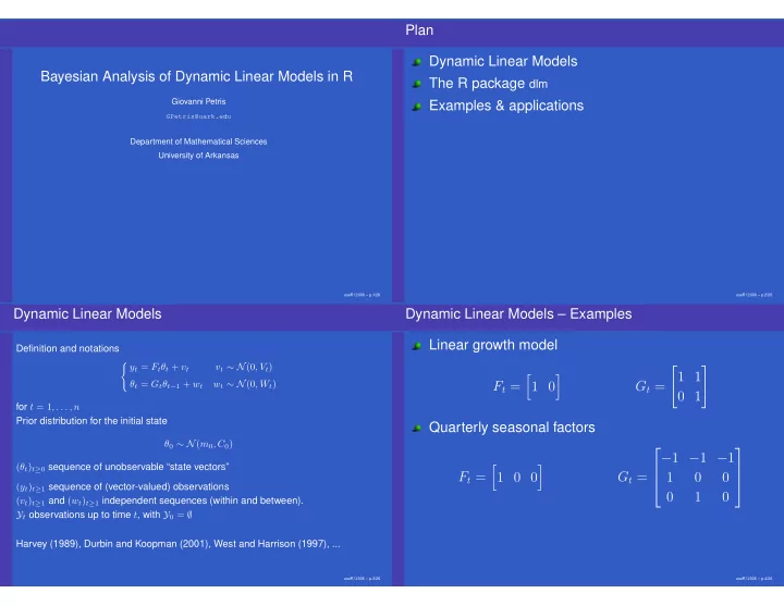
Plan Dynamic Linear Models Bayesian Analysis of Dynamic Linear Models in R The R package dlm Giovanni Petris Examples & applications GPetris@uark.edu Department of Mathematical Sciences University of Arkansas useR! 2006 p.1/26 useR!
Plan Dynamic Linear Models Bayesian Analysis of Dynamic Linear Models in R The R package dlm Giovanni Petris Examples & applications GPetris@uark.edu Department of Mathematical Sciences University of Arkansas useR! 2006 – p.1/26 useR! 2006 – p.2/26 Dynamic Linear Models Dynamic Linear Models – Examples Linear growth model Definition and notations � y t = F t θ t + v t v t ∼ N (0 , V t ) � � 1 1 � � θ t = G t θ t − 1 + w t w t ∼ N (0 , W t ) F t = 1 0 G t = 0 1 for t = 1 , . . . , n Prior distribution for the initial state Quarterly seasonal factors θ 0 ∼ N ( m 0 , C 0 ) − 1 − 1 − 1 ( θ t ) t ≥ 0 sequence of unobservable “state vectors” � � F t = G t = 1 0 0 1 0 0 ( y t ) t ≥ 1 sequence of (vector-valued) observations 0 1 0 ( v t ) t ≥ 1 and ( w t ) t ≥ 1 independent sequences (within and between). Y t observations up to time t , with Y 0 = ∅ Harvey (1989), Durbin and Koopman (2001), West and Harrison (1997), ... useR! 2006 – p.3/26 useR! 2006 – p.4/26
Dynamic Linear Models – Model composition Distributions of interest θ t |Y t filtering Linear growth plus seasonal component θ s |Y t s < t smoothing 1 1 0 0 0 θ s |Y t forecasting s > t 0 1 0 0 0 y s |Y t forecasting s > t � � F t = G t = 1 0 1 0 0 0 0 − 1 − 1 − 1 0 0 1 0 0 Possibly jointly, e.g. θ 1 , . . . , θ t |Y t 0 0 0 1 0 Every conditional distribution is Gaussian, identified by General model composition of n DLM’s mean and variance � � G t = BlockDiag( G (1) t , G (2) t , . . . , G ( n ) F (1) F (2) F ( n ) F t = ) . . . t t t t Kalman filter n V ( i ) W t = BlockDiag( W (1) , W (2) , . . . , W ( n ) � V t = ) t t t t i =1 useR! 2006 – p.5/26 useR! 2006 – p.6/26 Unknown parameters The R package dlm May be present in the matrices defining the DLM – The intended user evolution and observation equations or variance matrices is familiar with R, at least at a basic level Estimation: MLE, Bayes, other has some knowledge of Bayesian statistics, including the ideas of Gibbs sampling and Markov chain Monte Likelihood evaluation may by tricky – computational Carlo (no need to be an expert!) stability useR! 2006 – p.7/26 useR! 2006 – p.8/26
The generality dilemma Objects of class “dlm” Flexibility vs robustness and ease-of-use Constant models are defined in R as lists with Package dlm is flexible components FF, V, GG, W , with a class attribute equal to “dlm” Computational stability issues are dealt with using filtering Creators for common DLM’s are available and smoothing algorithms based on Singular Value > mod <- dlmModPoly(2) > names(mod) Decomposition [1] "m0" "C0" "FF" "V" "GG" "W" "JFF" "JV" "JGG" "JW" > mod$FF [,1] [,2] [1,] 1 0 > mod$GG [,1] [,2] [1,] 1 1 [2,] 0 1 > class(mod) [1] "dlm" useR! 2006 – p.9/26 useR! 2006 – p.10/26 Objects of class “dlm” – model composition Filtering & Smoothing dlm objects can be added together Recursive algorithms for filtering and smoothing are based on the SVD of the relevant covariance matrices > mod <- dlmModPoly(2) + dlmModSeas(4) Zhang and Li (1996) > mod$GG [,1] [,2] [,3] [,4] [,5] SVD of matrix H : H = USV ′ with U, V orthogonal, S [1,] 1 1 0 0 0 [2,] 0 1 0 0 0 diagonal [3,] 0 0 -1 -1 -1 For a nonnegative definite symmetric matrix, U = V , [4,] 0 0 1 0 0 S = D 2 [5,] 0 0 0 1 0 t − 1 U ′ C t − 1 = U t − 1 D 2 θ t − 1 |Y t − 1 ∼ N ( m t − 1 , C t − 1 ) , t − 1 t + W t = ˜ U t ˜ t ˜ R t = G t C t − 1 G ′ D 2 U ′ θ t |Y t − 1 ∼ N ( a t , R t ) , t → ˜ U t , ˜ U t − 1 , D t − 1 �− D t useR! 2006 – p.11/26 useR! 2006 – p.12/26
Maximum Likelihood MLE – Example Data: US quarterly log GDP from 1953 to 1995 ⇒ ⇒ ψ = Model = Loglikelihood Model: linear growth plus AR(2) Data and estimated trend To achieve a maximum of flexibility, the user has to explicitely specify the first step, ψ = ⇒ Model 8.6 8.4 R takes care of the evaluation of the Loglikelihood and of its maximization – via a call to optim 8.2 GDP 8.0 Warning : likelihood maximization is a tricky business!!! 7.8 7.6 7.4 1960 1970 1980 1990 Time useR! 2006 – p.13/26 useR! 2006 – p.14/26 MLE – Example Filtering & Smoothing – Example > buildGdp <- function(parm) { + trend <- dlmModPoly(2, dV=1e-10, dW=exp(parm[1:2])) > filt <- dlmFilter(gdp,modFit2) + z <- parm[3:4] / (1 + abs(parm[3:4])) + ar2 <- dlmModARMA(ar=c(sum(z),-prod(z)), sigma2=exp(parm[5])) > smooth <- dlmSmooth(filt) + return( trend + ar2 ) > plot(cbind(gdp,smooth$s[,1]), plot.type=’s’, lty=1:2, + } + ylab="GDP", main="Data and estimated trend") > mleGdp1 <- dlmMLE( gdp, parm=rep(0,5), build=buildGdp) > set.seed(4521) > mleGdp2 <- dlmMLE( gdp, parm=rep(0,5), build=buildGdp, method="SANN", + control=list(temp=20, tmax=25, maxit=20000)) > modFit1 <- buildGdp(mleGdp1$par) > dlmLL(gdp, modFit1) [1] 124.8836 > modFit2 <- buildGdp(mleGdp2$par) > dlmLL(gdp, modFit2) [1] -693.0615 useR! 2006 – p.15/26 useR! 2006 – p.16/26
Bayesian analysis How can i do it? For p (Θ n | α, Y n ) the package provides the function Θ t = ( θ 0 , . . . , θ t ) state vectors up to time t α = ( α 1 , . . . , α r ) dlmBSample , implementing the Forward Filtering Backward vector of unknown parameters Sampling algorithm Target posterior distribution p (Θ n , α |Y n ) Carter and Kohn (1994), Frühwirth-Schnatter (1994), Shephard (1994) Obtain a sample from the target distribution using the Gibbs sampler Generating from p ( α | Θ n , Y n ) is model-dependent – the generality dilemma strikes again! 1. p (Θ n | α, Y n ) 2. p ( α | Θ n , Y n ) R provides functions to generate from standard univariate distributions, dlm provides in addition a function to Step 2 may be broken down into several sub-steps generate from a Wishart distribution involving full conditional distributions of components of α If the full conditional distribution of α is nonstandard... useR! 2006 – p.17/26 useR! 2006 – p.18/26 If all else fail... arms! Example > bimodal <- function(x) { Adaptive Rejection Metropolis Sampling is a black-box + log(prod(dnorm(x,mean=3)) + prod(dnorm(x,mean=-3))) } algorithm to generate from a univariate continuous > y <- arms(c(-2,2), bimodal, distribution on a bounded support + function(x) all(x>(-10))*all(x<(10)), 500) Gilks, Best and Tan (1995) > plot(y, main="Mixture of bivariate Normals", asp=1) The package includes a multivariate extension of ARMS The user needs to write two functions in R: one to evaluate the logdensity of the target the other to evaluate the indicator function of the support The rest is taken care of by the function arms useR! 2006 – p.19/26 useR! 2006 – p.20/26
Multivariate ARMS Application 4 6 2 4 0 2 −2 x 2 M1 0 −4 GNP −2 1978 1980 1982 1984 1986 1988 −4 −6 Data: bivariate quarterly time series of differenced log of −6 −4 −2 0 2 4 6 seasonally adjusted real US money “M1” and GNP . x 1 useR! 2006 – p.21/26 useR! 2006 – p.22/26 Model Gibbs Sampler Seemingly Unrelated Time Series – Local level Generate in turn F t = I 2 , G t = I 2 , 1. p (Θ n | V, q, Y n ) — Forward Filtering Backward V t = V, W t = q · V Sampling 2. p ( V | Θ n , q, Y n ) — Inverse Wishart ) ′ θ t = ( µ M 1 , µ GNP t t 3. p ( q | Θ n V, Y n ) — ARMS Prior: V ∼ IW , q ∼ Unif( ǫ, M ) useR! 2006 – p.23/26 useR! 2006 – p.24/26
Estimated levels Recap User-friendly, flexible package for DLM analysis 4 Fast and numerically stable Focus on Bayesian, but also includes MLE 2 A preliminary version of the package dlm can be downloaded at the URL 0 −2 http://definetti.uark.edu/~gpetris/DLM M1 − observed −4 M1 − Bayes estimate of level GNP − observed GNP − Bayes estimate of level 1978 1980 1982 1984 1986 1988 useR! 2006 – p.25/26 useR! 2006 – p.26/26
Recommend
More recommend
Explore More Topics
Stay informed with curated content and fresh updates.
