1. Introduction limit reductions: energy, environmental and safety - PDF document
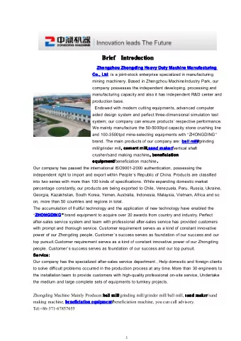
Using naturalistic driving data to evaluate speed 1. Introduction limit reductions: energy, environmental and safety Motivation assessment Significant impacts of transport sector: o Energy consumption ( security of supply) o GHG
Using naturalistic driving data to evaluate speed 1. Introduction limit reductions: energy, environmental and safety Motivation assessment • Significant impacts of transport sector: o Energy consumption ( → security of supply) o GHG emissions ( → global warming) Patrícia Baptista, Marta Faria, Gonçalo Duarte o Local pollutants ( → air quality, health) o Accidents ( → injuries, fatalities) 31 st ICTCT conference o Etc. 25 - 26 October, 2018 Porto, Portugal CO 2 emissions 2 1. Introduction 1. Introduction Motivation Motivation • Significant impacts of transport sector: • Alternative options on urban mobility: o Energy consumption ( → security of supply) o Redesign of infrastructure → reduction of speed limits o GHG emissions ( → global warming) o Local pollutants ( → air quality, health) o Accidents ( → injuries, fatalities) o Etc. • Alternative options on urban mobility: o Cross-modal electrification o Transport system integration coupled with Mobility-as-a-Service (MaaS) to promote modal shift o Redesign of transport infrastructure (urban plazas, reduction of speed limits, etc.) o Etc. 3 4
1. Introduction 1. Introduction Motivation Motivation • Alternative options on urban mobility: • Alternative options on urban mobility: o Redesign of infrastructure → reduction of speed limits o Redesign of infrastructure → reduction of speed limits � Reduce accident risk � Reduce accident risk � Improve the urban environment for pedestrians and biker � Improve the urban environment for pedestrians and bikers � Promotion of MaaS products (bike, scooter-sharing, etc.) � Promotion of MaaS products (bike, scooter-sharing, etc.) 5 6 1. Introduction 2. Data and Methods Objective 2.1. Data collection • Assess the impacts of reducing speed limits on a one-vehicle/driver • 12 drivers under real world driving conditions perspective: • Data collection in Lisbon metropolitan area • 1 month of data (September 2016), corresponding to 16412 km and 441 hours of o Using real world driving data (naturalistic driving data) driving Driver number GENRE AGE_GROUP EXPERIENCE FUEL_TYPE DISPLACEMENT CAR_DATE • Vehicles’ characteristics: 1 Female 35-49 years 10-24 years Diesel 1598 2011 2 Male 25-34 years 10-24 years Diesel 1598 2013 o Considering the type of road where the vehicle drives 3 Male 35-49 years 25-49 years Diesel 1461 2008 4 Female 25-34 years 10-24 years Diesel 1461 2008 5 Female 35-49 years 25-49 years Diesel 1560 2010 6 Female 50-64 years 25-49 years Diesel 1995 2013 o Case study: Lisbon Metropolitan area 7 Female 35-49 years 10-24 years Gasoline 1242 2006 8 Female 35-49 years 10-24 years Gasoline 1198 2006 9 Female 35-49 years 25-49 years Diesel 1493 2005 10 Male 35-49 years 25-49 years Diesel 1598 2012 11 Male 25-34 years 10-24 years Diesel 1968 2008 12 Male 35-49 years 10-24 years Diesel 1991 2007 7 8
2. Data and Methods 2. Data and Methods 2.1. Data collection 2.2. Quantification of energy consumption Analysis of 1 Hz driving data to assess: • Vehicle Specific Power – methodology to correlate vehicle dynamics with fuel use, pollutant emissions VSP accounts for driver aggressiveness d through speed and dt �E Kinetic + E Potential � + F Rolling ∙ v + F Aerod ynamic ∙ v VSP = = acceleration m = � ∙ �� ∙ �1 + ! " � + # ∙ $%&�'� + ( )*++ , + ( -%.* ∙ � 3 9 10 2. Data and Methods 2. Data and Methods 2.2. Quantification of energy consumption 2.2. Quantification of energy consumption 7.6 l/100km Measured drive cycle Measured drive cycle Fuel consumption VSP time per VSP mode distribution Per vehicle 11 Per vehicle 12
2. Data and Methods 2. Data and Methods 2.2. Quantification of energy consumption 7.6 l/100km 2.3. Model development – drive cycle adjustment VSP time Measured drive cycle Fuel consumption Original drive cycle From GPS → type pf road per VSP mode distribution Level 4 Level 3 Level 2 Level 4 Reverse geocoding for each second of driving: VSP time distribution Another drive cycle -Level 1 – arterial streets -Level 2 – minor arterial streets -Level 3 – distributor and collector streets -Level 4 – local streets 6.9 l/100km Per driver Per vehicle 13 14 2. Data and Methods 2. Data and Methods 2.3. Model development – drive cycle adjustment 2.3. Model development – drive cycle adjustment Original drive cycle From GPS → type pf road Original drive cycle From GPS → type pf road Level 4 Level 3 Level 2 Level 4 Level 4 Level 3 Level 2 Level 4 Original 1 month driving data (speed, altitude) New drive cycle with modified speed limits Second-by-second power requirement (VSP) Adjustment of speed and acceleration to fulfill criteria by maintaining: Verification of speed criteria: -Total distance - Maximum speed (km/h) according to road level -Stops along road infrastructure -Power requirements Per driver Per driver 15 16
2. Data and Methods 2. Data and Methods 2.4. Definition of scenarios 2.4. Application of scenarios 4 scenarios were considered and compared to the real-world driving cycle (BAU): Application of scenarios to assess: Speed limit (km/h) BAU Sc 1. Sc 2. Sc 3. Sc 4. • total driving time (for same L1 - 120 90 90 90 distance) Street L2 - 50 50 50 50 • average speed (km/h) level L3 - 50 50 50 30 • acceleration L4 - 50 50 30 30 • energy consumption (g/s and l/100km) • energy consumption reduction potential (%) 17 18 3. Results 3. Results Average of all drivers Average of all drivers Scenarios Sc. 1 Sc. 2 Sc. 3 Sc. 4 Scenarios Sc. 1 Sc. 2 Sc. 3 Sc. 4 Distance (km) Difference to BAU (%) 0% 0% 0% 0% Distance (km) Difference to BAU (%) 0% 0% 0% 0% Difference to BAU (%) 1% 17% 41% 44% Difference to BAU (%) 1% 17% 41% 44% Time (h) Time (h) Difference in hours 0.30 7.57 18.13 18.90 Difference in hours 0.30 7.57 18.13 18.90 Difference to BAU (%) -58% -1340% -2641% -2787% Difference to BAU (%) -58% -1340% -2641% -2787% Average Speed (km/h) Average Speed (km/h) Difference in km/h -0.29 -5.58 -10.51 -10.92 Difference in km/h -0.29 -5.58 -10.51 -10.92 Maximum speed (km/h) Difference to BAU (%) -17% -38% -38% -38% Maximum speed (km/h) Difference to BAU (%) -17% -38% -38% -38% acc slope >0 Difference to BAU (%) -8% -52% -125% -104% acc slope >0 Difference to BAU (%) -8% -52% -125% -104% acc slope <0 Difference to BAU (%) -2% -103% -176% -185% acc slope <0 Difference to BAU (%) -2% -103% -176% -185% Average positive VSP (W/kg) Difference to BAU (%) -4% -35% -50% -53% Average positive VSP (W/kg) Difference to BAU (%) -4% -35% -50% -53% Energy consumption (MJ/km) Difference to BAU (%) -13% -2% 5% 7% Energy consumption (MJ/km) Difference to BAU (%) -13% -2% 5% 7% • Very significant reductions in acceleration (connected with driver • Up to 11 km/h reduction in Scenario 4, with corresponding increase in travel time (44%) aggressiveness), mostly noticeable in deceleration events 19 20
3. Results 3. Results Average of all drivers Results per driver Scenarios Sc. 1 Sc. 2 Sc. 3 Sc. 4 Distance (km) Difference to BAU (%) 0% 0% 0% 0% • D5, 6, 10, 11 and 12 Difference to BAU (%) 1% 17% 41% 44% Time (h) with higher reductions Difference in hours 0.30 7.57 18.13 18.90 in Avg. Speed Difference to BAU (%) -58% -1340% -2641% -2787% Average Speed (km/h) Difference in km/h -0.29 -5.58 -10.51 -10.92 Maximum speed (km/h) Difference to BAU (%) -17% -38% -38% -38% acc slope >0 Difference to BAU (%) -8% -52% -125% -104% • Association with the acc slope <0 Difference to BAU (%) -2% -103% -176% -185% context and Average positive VSP (W/kg) Difference to BAU (%) -4% -35% -50% -53% conditions of driving Energy consumption (MJ/km) Difference to BAU (%) -13% -2% 5% 7% Scenario 1 presents slight impacts → understandable at urban scale; • Scenario 3 and 4 have very similar impacts 21 22 3. Results 3. Results Energy impacts per driver Energy impacts per driver • This change in drive Fuel consumption cycle is reflected in modifications in Local pollutants energy consumption (HC, CO, NO x , PM) • Sc. 1 results in reduction in energy consumption, but Opportunity for speed limitation in Sc electric mobility for 2, 3 and 4 result in mitigating impacts up to 15% increases 23 24
Recommend


More recommend
Explore More Topics
Stay informed with curated content and fresh updates.