(1, )-Evolution Strategy with Cumulative Step size Adaptation on - PowerPoint PPT Presentation
(1, )-Evolution Strategy with Cumulative Step size Adaptation on linear cost functions Adrien Coutoux, Auger Anne, Hansen Nikolaus INRIA Saclay - Ile-de-France, Project team TAO (1, )-Evolution Strategy with Cumulative Step size
(1, λ )-Evolution Strategy with Cumulative Step size Adaptation on linear cost functions Adrien Couëtoux, Auger Anne, Hansen Nikolaus INRIA Saclay - Ile-de-France, Project team TAO (1, λ )-Evolution Strategy with Cumulative Step size Adaptation on linear cost functions - Adrien Couëtoux – 25/01/10
Problem statement Continuous optimization: minimization of a cost f(x), x ∈ R d depending on , d being the dimension of the search space, that is unbounded. We study the behavior of one evolutionary strategy, the (1, λ )- ES with Cumulative Step size Adaptation (CSA) We limit our study to the case where the cost function f(.) is linear. This case is important because most cost functions can be approximated, on small intervals, by linear functions. (1, λ )-Evolution Strategy with Cumulative Step size Adaptation on linear cost functions - Adrien Couëtoux – 25/01/10
Problem statement - (1, λ )-Evolution Strategy Representation in 2-D, with the cost function f(x 1 ,x 2 )=x 1 from one parent, we generate λ off-springs, and select one of them as the next parent. x 2 Candidates x 1 Parent (1, λ )-Evolution Strategy with Cumulative Step size Adaptation on linear cost functions - Adrien Couëtoux – 25/01/10
Problem statement - (1, λ )-Evolution Strategy Representation in 2-D, with the cost function f(x 1 ,x 2 )=x 1 from one parent, we generate λ off-springs, and select one of them as the next parent. x 2 Candidates Parent x 1 Selected Candidate (1, λ )-Evolution Strategy with Cumulative Step size Adaptation on linear cost functions - Adrien Couëtoux – 25/01/10
Problem statement - Cumulative Step size Adaptation Given a point X in the search space, one standard way of generating a candidate solution is the following: ( ) X candidate ~ X + σ N 0, I d σ being called the step size In our case, the cost function is linear, and the search space is unbounded. This means that the optimal solution is infinite. Hence, we want our population to diverge towards the optimal direction (this direction being the opposite of the gradient of f(.)). To have a population that quickly moves toward the optimum, we need to have a large step size. (1, λ )-Evolution Strategy with Cumulative Step size Adaptation on linear cost functions - Adrien Couëtoux – 25/01/10
Our goals We want to show that CSA is proficient on linear functions. This means that we have to make sure that the step size is growing, and that our population moves toward the right direction. For practical reasons, we will study the series ( ) − ln σ n ( ) ln σ n + 1 rather than the step size itself. To simplify our computations, we consider the case where the cost function is f(x 1 …,x d )=x 1 . (1, λ )-ES is rotational invariant, and the gradient of a linear function is a constant vector. Hence, our results do not suffer from this simplification. (1, λ )-Evolution Strategy with Cumulative Step size Adaptation on linear cost functions - Adrien Couëtoux – 25/01/10
CSA algorithm Parameters 0<c<1 (usually between 1/d 1/2 and 1/d); it represents the weight of the past of the search in the update procedure λ (number of candidates sampled at each iteration) X 0 the initial parent, σ 0 >0 the initial step size and p 0 a vector of the search space, the initial path (usually 0 search_space ) When at the n th iteration, given the current population X n in S, step size σ n and path p n : We sample λ candidates (X n,i ) 1 ≤ i ≤λ , independent and identically distributed with ( ) X n , i ~ X n + σ n N 0, I d We select the one member that minimizes the cost function: X n+1 =argmin 1 ≤ i ≤λ {f(X n,i )} (=min{X n,i,1 } in our case ) (1, λ )-Evolution Strategy with Cumulative Step size Adaptation on linear cost functions - Adrien Couëtoux – 25/01/10
CSA algorithm – update of the step size and the path We update the path: ( ) p n + ( ) Y n p n + 1 = 1 − c c 2 − c with Y n = X n + 1 − X n σ n We update the step size: 2 p n + 1 σ n + 1 = σ n exp c − 1 2 d (1, λ )-Evolution Strategy with Cumulative Step size Adaptation on linear cost functions - Adrien Couëtoux – 25/01/10
Simulations-logarithm of the step size Evolution of the logarithm of the step size, as a function of the number of iterations (d=20, λ =15, c=0.05): (1, λ )-Evolution Strategy with Cumulative Step size Adaptation on linear cost functions - Adrien Couëtoux – 25/01/10
Study of the step size We study the growth of the step size, through the difference between the logarithm of the updated step size and the one of the current step size: 2 p n + 1 ) = c ( ) − ln σ n ( ln σ n + 1 − 1 2 d ( ) = d 2 Note that . We compare the expectation of the ( ) E N 0, I d path to its expectation if the selection was done completely randomly (i.e. “random search”). This clearly suggest that to obtain results on the step size, we first need to study the path, or at least its squared norm. (1, λ )-Evolution Strategy with Cumulative Step size Adaptation on linear cost functions - Adrien Couëtoux – 25/01/10
Theoretical results-How does the path evolves? ( ) p n + ( ) Y n p n + 1 = 1 − c c 2 − c Remember: Looks like a Markov chain… (1, λ )-Evolution Strategy with Cumulative Step size Adaptation on linear cost functions - Adrien Couëtoux – 25/01/10
Theoretical results-How does the path evolves? ( ) p n + ( ) Y n p n + 1 = 1 − c c 2 − c Remember: Looks like a Markov chain… Selection only relies on the first coordinate. The selected member is the one with the lowest first coordinate, among λ independent and identically distributed random variables. is the first order N 1: λ statistic of λ normal variables. We can show that indeed (p n ) n ≥ 0 is a Markov chain, and that: N 1: λ N 2 λ − 1 ( ) ϕ 1: λ ( x ) = λϕ ( x ) 1 − Φ ( x ) Y = N d (1, λ )-Evolution Strategy with Cumulative Step size Adaptation on linear cost functions - Adrien Couëtoux – 25/01/10
Theoretical results-How does the path evolves? ( ) p n + ( ) Y n p n + 1 = 1 − c c 2 − c Remember: Looks like a Markov chain… Selection only relies on the first coordinate. The selected member is the one with the lowest first coordinate, among λ independent and identically distributed random variables. is the first order N 1: λ statistic of λ normal variables. We can show that indeed (p n ) n ≥ 0 is a Markov chain, and that: N 1: λ Independent of n N 2 λ − 1 ( ) ϕ 1: λ ( x ) = λϕ ( x ) 1 − Φ ( x ) Y = N d (1, λ )-Evolution Strategy with Cumulative Step size Adaptation on linear cost functions - Adrien Couëtoux – 25/01/10
Expectation of the squared norm of the path 2 Using nothing but the previous equations, we prove that p n + 1 has a limit in expectation, and we find the following explicit expression ( ) ) + 2 1 − c 2 = d − 1 + E N 1: λ ( 2 2 ( ) L p : = lim n →∞ E p n E N 1: λ c ( ) − 1 ≥ 0 2 E N 1: λ and In our simulations, with d=20, c=0.01, and λ =15, this gives L p =144.4945 (1, λ )-Evolution Strategy with Cumulative Step size Adaptation on linear cost functions - Adrien Couëtoux – 25/01/10
Expectation of the squared norm of the path 2 Using nothing but the previous equations, we prove that p n + 1 has a limit in expectation, and we find the following explicit expression ( ) ) + 2 1 − c 2 = d − 1 + E N 1: λ ( 2 2 ( ) L p : = lim n →∞ E p n E N 1: λ c ( ) − 1 ≥ 0 2 E N 1: λ and In our simulations, with d=20, c=0.01, and λ =15, this gives L p =144.4945 Why is it interesting? (1, λ )-Evolution Strategy with Cumulative Step size Adaptation on linear cost functions - Adrien Couëtoux – 25/01/10
Expectation of the squared norm of the path 2 Using nothing but the previous equations, we prove that p n + 1 has a limit in expectation, and we find the following explicit expression ( ) ) + 2 1 − c 2 = d − 1 + E N 1: λ ( 2 2 ( ) L p : = lim n →∞ E p n E N 1: λ c ( ) − 1 ≥ 0 2 E N 1: λ and In our simulations, with d=20, c=0.01, and λ =15, this gives L p =144.4945 Why is it interesting? 2 p n + 1 ) = c ( ) − ln σ n ( ln σ n + 1 − 1 2 d (1, λ )-Evolution Strategy with Cumulative Step size Adaptation on linear cost functions - Adrien Couëtoux – 25/01/10
2 Simulations- p n + 1 Evolution of the squared norm of the path (blue), and of its expectation (red), with respect to n (d=20, λ =15, c=0.05) (1, λ )-Evolution Strategy with Cumulative Step size Adaptation on linear cost functions - Adrien Couëtoux – 25/01/10
Maximum number of iterations to obtain a growing step size If we add the (very reasonable) assumption that, as one usually does, p 0 is initialized such that E(p 0 )=0, we can provide an upper bound to the number of iterations required for the squared norm of the path to reach a certain level. For all, for all n>M, 2 ≥ d + c 2 − c ( ) > d ( ) − 1 2 ( ) E N 1: λ E p n d with M = = 20.5426 ( ) ( ) − 1 2 ( ) E N 1: λ c 2 − c (1, λ )-Evolution Strategy with Cumulative Step size Adaptation on linear cost functions - Adrien Couëtoux – 25/01/10
Recommend
More recommend
Explore More Topics
Stay informed with curated content and fresh updates.
