1.2 Row Reduction and Echelon Forms McDonald Fall 2018, MATH 2210Q - PDF document

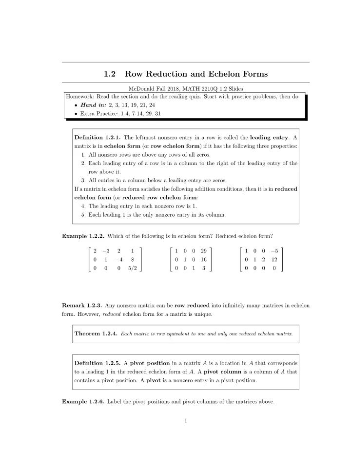
1.2 Row Reduction and Echelon Forms McDonald Fall 2018, MATH 2210Q 1.2 Slides Homework: Read the section and do the reading quiz. Start with practice problems, then do ❼ Hand in: 2, 3, 13, 19, 21, 24 ❼ Extra Practice: 1-4, 7-14, 29, 31 Definition 1.2.1. The leftmost nonzero entry in a row is called the leading entry . A matrix is in echelon form (or row echelon form ) if it has the following three properties: 1. All nonzero rows are above any rows of all zeros. 2. Each leading entry of a row is in a column to the right of the leading entry of the row above it. 3. All entries in a column below a leading entry are zeros. If a matrix in echelon form satisfies the following addition conditions, then it is in reduced echelon form (or reduced row echelon form : 4. The leading entry in each nonzero row is 1. 5. Each leading 1 is the only nonzero entry in its column. Example 1.2.2. Which of the following is in echelon form? Reduced echelon form?       2 − 3 2 1 1 0 0 29 1 0 0 − 5 0 1 − 4 8 0 1 0 16 0 1 2 12             0 0 0 5 / 2 0 0 1 3 0 0 0 0 Remark 1.2.3. Any nonzero matrix can be row reduced into infinitely many matrices in echelon form. However, reduced echelon form for a matrix is unique. Theorem 1.2.4. Each matrix is row equivalent to one and only one reduced echelon matrix. Definition 1.2.5. A pivot position in a matrix A is a location in A that corresponds to a leading 1 in the reduced echelon form of A . A pivot column is a column of A that contains a pivot position. A pivot is a nonzero entry in a pivot position. Example 1.2.6. Label the pivot positions and pivot columns of the matrices above. 1

Example 1.2.7. Row reduce the matrix A to echelon form and locate pivot columns.   0 − 3 − 6 4 9  − 1 − 2 − 1 3 1    A =   − 2 − 3 0 3 − 1     1 4 5 − 9 − 7 2

Procedure 1.2.8 (Row Reduction Algorithm) . To transform a matrix into echelon form: 1. Begin with the leftmost nonzero column. This is a pivot column. The pivot position is at the top. 2. Select a non-zero entry in the pivot column as a pivot, and interchange rows if necessary to move this entry into the pivot position. 3. Use row replacement to create zeros in all positions below the pivot. 4. Cover (ignore) the row containing the pivot positions and all rows, if any, above it. Apply steps 1-3 to the submatrix that remains. Repeat until there are no more nonzero rows to modify. If you want reduced echelon form, add one more step 5. Beginning with the rightmost pivot and working upward and to the left, create zeros above each pivot. If a pivot is not 1, make it 1 by scaling. Example 1.2.9. Apply elementary row operations to transform the following matrix into echelon form, and then reduced echelon form.   0 3 − 6 6 4 − 5 3 − 7 8 − 5 8 9     3 − 9 12 − 9 6 15 Definition 1.2.10. Steps 1-4 above are called the forward phase of the row reduction algorithm. Step 5 is called the backward phase. 3

Example 1.2.11. Find the general solution of a linear system whose augmented matrix can be reduced to the matrix below.   1 0 − 5 1 0 1 1 4     0 0 0 0 Definition 1.2.12. The variables corresponding to pivot columns of a matrix are called basic variables , the other variables are called free variables . Remark 1.2.13. Whenever a system is consistent, the solution set can be described explicitly by solving the reduced system of equations for the basic variables in terms of the free variables. Example 1.2.14. Find the general solution of a system whose augmented matrix is reduced to   1 6 2 − 5 − 2 − 4 0 0 2 − 8 − 1 3     0 0 0 0 1 7 Remark 1.2.15. The solutions in these examples are called parametric descriptions . Finding a general solution means finding a parametric description of the solution set, or determining that it is empty. If a system is inconsistent, then the solution set has no parametric representation. 4

Example 1.2.16. Solve the following system: x 1 − 7 x 2 + 2 x 3 − 5 x 4 + 8 x 5 = 10 x 2 − 3 x 3 + 3 x 4 + x 5 = − 5 x 4 − x 5 = 4 Remark 1.2.17. The method we used above is called back substitution . When we reduce to reduced echelon form, this is handled by the backward phase and reduces the likelihood of errors. Example 1.2.18. Determine the existence and uniqueness of the solutions to the system 3 x 2 − 6 x 3 + 6 x 4 + 4 x 5 = − 5 3 x 1 − 7 x 2 + 8 x 3 − 5 x 4 + 8 x 5 = 9 3 x 1 − 9 x 2 + 12 x 3 − 9 x 4 + 6 x 5 = 15 Theorem 1.2.19. A linear system is consistent if and only if the rightmost column of the augmented matrix is not a pivot column. If a linear system is consistent, then the solution set contains either (i) a unique solution, where there are no free variables, or (ii) infinitely many solutions, when there is at least one free variable. 5

Using the theorem, and the rest of this section, we have the following procedure to find and describe all the solutions of a linear system. Procedure 1.2.20 (Using Row Reduction to Solve a Linear System) . 1. Write the augmented matrix of the system. 2. Use the row reduction algorithm to write the matrix in echelon form. If the system is inconsistent, stop, there are no solutions; otherwise, go to the next step. 3. Use the row reduction algorithm to write the matrix in reduced echelon form. 4. Write the system of equations corresponding to the reduced matrix. 5. Solve each basic variable in terms of any free variables. 6