Reducing Data Dimension Recommended reading: Bishop, chapter 3.6, - PowerPoint PPT Presentation

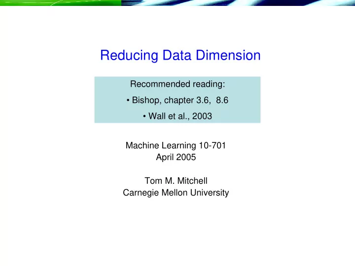
Reducing Data Dimension Recommended reading: • Bishop, chapter 3.6, 8.6 • Wall et al., 2003 Machine Learning 10-701 April 2005 Tom M. Mitchell Carnegie Mellon University

Outline • Feature selection – Single feature scoring criteria – Search strategies • Unsupervised dimension reduction using all features – Principle Components Analysis – Singular Value Decomposition – Independent components analysis • Supervised dimension reduction – Fisher Linear Discriminant – Hidden layers of Neural Networks

Dimensionality Reduction Why? • Learning a target function from data where some features are irrelevant • Wish to visualize high dimensional data • Sometimes have data whose “intrinsic” dimensionality is smaller than the number of features used to describe it - recover intrinsic dimension

Supervised Feature Selection

Supervised Feature Selection Problem: Wish to learn f: X � Y, where X=<X 1 , …X N > But suspect not all X i are relevant Approach: Preprocess data to select only a subset of the X i • Score each feature, or subsets of features – How? • Search for useful subset of features to represent data – How?

Scoring Individual Features X i Common scoring methods: • Training or cross-validated accuracy of single-feature classifiers f i : X i � Y • Estimated mutual information between X i and Y : χ 2 statistic to measure independence between X i and Y • • Domain specific criteria – Text: Score “stop” words (“the”, “of”, …) as zero – fMRI: Score voxel by T-test for activation versus rest condition – …

Choosing Set of Features Common methods: Forward1: Choose the n features with the highest scores Forward2: – Choose single highest scoring feature X k – Rescore all features, conditioned on X k being selected • E.g, Score(X i )= Accuracy({X i , X k }) • E.g., Score(X i ) = I(X i ,Y |X k ) – Repeat, calculating new conditioned scores on each iteration

Choosing Set of Features Common methods: Backward1: Start with all features, delete the n with lowest scores Backward2: Start with all features, score each feature conditioned on assumption that all others are included. Then: – Remove feature with the lowest (conditioned) score – Rescore all features, conditioned on the new, reduced feature set – Repeat

Feature Selection: Text Classification [Rogati&Yang, 2002] Approximately 10 5 words in English IG=information gain, chi= χ 2 , DF=doc frequency,

Impact of Feature Selection on Classification of fMRI Data [Pereira et al., 2005] Accuracy classifying category of word read by subject Voxels scored by p-value of regression to predict voxel value from the task

Summary: Supervised Feature Selection Approach: Preprocess data to select only a subset of the X i • Score each feature – Mutual information, prediction accuracy, … • Find useful subset of features based on their scores – Greedy addition of features to pool – Greedy deletion of features from pool – Considered independently, or in context of other selected features Always do feature selection using training set only (not test set!) – Often use nested cross-validation loop: • Outer loop to get unbiased estimate of final classifier accuracy • Inner loop to test the impact of selecting features

Unsupervised Dimensionality Reduction

Unsupervised mapping to lower dimension Differs from feature selection in two ways: • Instead of choosing subset of features, create new features (dimensions) defined as functions over all features • Don’t consider class labels, just the data points

Principle Components Analysis • Idea: – Given data points in d-dimensional space, project into lower dimensional space while preserving as much information as possible • E.g., find best planar approximation to 3D data • E.g., find best planar approximation to 10 4 D data – In particular, choose projection that minimizes the squared error in reconstructing original data

PCA: Find Projections to Minimize Reconstruction Error Assume data is set of d-dimensional vectors, where nth vector is We can represent these in terms of any d orthogonal basis vectors u 1 PCA: given M<d. Find u 2 that minimizes x 2 where Mean x 1

PCA u 1 u 2 PCA: given M<d. Find x 2 that minimizes x 1 where Note we get zero error if M=d. Therefore, This minimized when u i is eigenvector of Σ, i.e., when: Covariance matrix:

PCA u 1 u 2 x 2 Minimize x 1 Eigenvector of Σ Eigenvalue PCA algorithm 1: 1. X � Create N x d data matrix, with one row vector x n per data point 2. X � subtract mean x from each row vector x n in X 3. Σ � covariance matrix of X 4. Find eigenvectors and eigenvalues of Σ 5. PC’s � the M eigenvectors with largest eigenvalues

PCA Example mean First eigenvector Second eigenvector

PCA Example Reconstructed data using only first eigenvector (M=1) mean First eigenvector Second eigenvector

Very Nice When Initial Dimension Not Too Big What if very large dimensional data? • e.g., Images (d ≥ 10^4) Problem: • Covariance matrix Σ is size (d x d) • d=10 4 � | Σ | = 10 8 Singular Value Decomposition (SVD) to the rescue! • pretty efficient algs available, including Matlab SVD • some implementations find just top N eigenvectors

SVD Data X , one Rows of V T are unit US gives S is diagonal, row per data coordinates length eigenvectors of S k > S k+1 , point 2 is kth of rows of X X T X . S k in the space largest If cols of X have zero of principle eigenvalue mean, then X T X = c Σ components and eigenvects are the Principle Components [from Wall et al., 2003]

Singular Value Decomposition To generate principle components: • Subtract mean from each data point, to create zero-centered data • Create matrix X with one row vector per (zero centered) data point • Solve SVD: X = USV T • Output Principle components: columns of V (= rows of V T ) – Eigenvectors in V are sorted from largest to smallest eigenvalues 2 giving eigenvalue for kth eigenvector – S is diagonal, with s k

Singular Value Decomposition To project a point (column vector x ) into PC coordinates: V T x If x i is i th row of data matrix X , then • (i th row of US) = V T x i T • (US) T = V T X T To project a column vector x to M dim Principle Components subspace, take just the first M coordinates of V T x

Independent Components Analysis • PCA seeks directions < Y 1 … Y M > in feature space X that minimize reconstruction error • ICA seeks directions < Y 1 … Y M > that are most statistically independent . I.e., that minimize I(Y), the mutual information between the Y j : Which maximizes their departure from Gaussianity!

Independent Components Analysis • ICA seeks to minimize I(Y), the mutual information between the Y j : … … • Example: Blind source separation – Original features are microphones at a cocktail party – Each receives sounds from multiple people speaking – ICA outputs directions that correspond to individual speakers

Supervised Dimensionality Reduction

1. Fisher Linear Discriminant • A method for projecting data into lower dimension to hopefully improve classification • We’ll consider 2-class case Project data onto vector that connects class means?

Fisher Linear Discriminant Project data onto one dimension, to help classification Define class means: Could choose w according to: Instead, Fisher Linear Discriminant chooses:

Fisher Linear Discriminant Project data onto one dimension, to help classification Fisher Linear Discriminant : is solved by : Where S W is sum of within-class covariances:

Fisher Linear Discriminant Fisher Linear Discriminant : Is equivalent to minimizing sum of squared error if we assume target values are not +1 and -1, but instead N/N 1 and –N/N 2 Where N is total number of examples , N i is number in class i Also generalized to K classes (and projects data to K-1 dimensions)

Summary: Fisher Linear Discriminant • Choose n-1 dimension projection for n-class classification problem • Use within-class covariances to determine the projection • Minimizes a different sum of squared error function

2. Hidden Layers in Neural Networks When # hidden units < # inputs, hidden layer also performs dimensionality reduction. Each synthesized dimension (each hidden unit) is logistic function of inputs Hidden units defined by gradient descent to (locally) minimize squared output classification/regression error Also allow networks with multiple hidden layers � highly nonlinear components (in contrast with linear subspace of Fisher LD, PCA)

Training neural network to minimize reconstruction error

Cognitive Neuroscience Models Based on ANN’s [McClelland & Rogers, Nature 2003]