Week 3: Linear Regression Instructor: Sergey Levine 1 Recap In - - PDF document

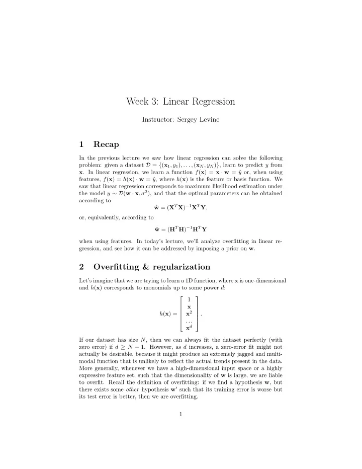
Week 3: Linear Regression

Instructor: Sergey Levine

1 Recap

In the previous lecture we saw how linear regression can solve the following problem: given a dataset D = {(x1, y1), . . . , (xN, yN)}, learn to predict y from

• x. In linear regression, we learn a function f(x) = x · w = ˆ

y or, when using features, f(x) = h(x) · w = ˆ y, where h(x) is the feature or basis function. We saw that linear regression corresponds to maximum likelihood estimation under the model y ∼ D(w · x, σ2), and that the optimal parameters can be obtained according to ˆ w = (XT X)−1XT Y,

• r, equivalently, according to

ˆ w = (HT H)−1HT Y when using features. In today’s lecture, we’ll analyze overfitting in linear re- gression, and see how it can be addressed by imposing a prior on w.

2 Overfitting & regularization

Let’s imagine that we are trying to learn a 1D function, where x is one-dimensional and h(x) corresponds to monomials up to some power d: h(x) =       1 x x2 . . . xd       . If our dataset has size N, then we can always fit the dataset perfectly (with zero error) if d ≥ N − 1. However, as d increases, a zero-error fit might not actually be desirable, because it might produce an extremely jagged and multi- modal function that is unlikely to reflect the actual trends present in the data. More generally, whenever we have a high-dimensional input space or a highly expressive feature set, such that the dimensionality of w is large, we are liable to overfit. Recall the definition of overfitting: if we find a hypothesis w, but there exists some other hypothesis w′ such that its training error is worse but its test error is better, then we are overfitting. 1

In linear regression, one of the most recognizable symptoms of overfitting is the existence of very large values in w. This would happen, for example, when erroneously fitting a high-degree polynomial with near-perfect accuracy to a noisy dataset. Note that this overfitting is quite similar to something we discussed last week in the context of maximum likelihood estimation: if we flip a coin and “accidentally” observe heads five times in a row, MLE might lead us to conclude the coin would always come up heads. But that is unreasonable. Question. How can we mitigate overfitting in linear regression? Answer. Same as last week, we can switch from MLE to a Bayesian approach, and compute the maximum a posteriori (MAP) estimate of the parameters w

• instead. This involves imposing a prior on w: our reasonable prior belief about

what the parameters should be, before we’ve even seen the data. A reasonable prior belief is that the parameters w should be small: this would prevent the sort of huge parameters we might see when fitting a high- degree polynomial with zero error. Question. What kind of distribution might be suitable for representing the prior on w? Answer. Since each entry in w is continuous, real-valued, and unconstrained, the Gaussian distribution is a good choice. In general, we could place a full multivariate Gaussian prior on the entire vector w, but for now let’s assume that we’ll place an independent Gaussian prior on each dimension of w, with prior mean zero and prior variance σ2

0, such that

log p(w) = − 1 2σ2

d

• j=1

w2

j + const.

This means that for each dimension j of w, we have wj ∼ N(0, σ2

0).1 Combining

this prior with the likelihood, we get log p(w|D) = − 1 2σ2

N

• i=1

(yi − xi · w)2 − 1 2σ2

d

• j=1

w2

j + const.

From the form of this likelihood, we can see that the posterior is also Gaussian. Just like before, we can compute the derivative of this quantity and set it to zero to determine the optimal weights: d dw  − 1 2σ2

N

• i=1

(yi − xi · w)2 − 1 2σ2

d

• j=1

w2

j

  = 1 σ2

N

• i=1

xi(yi − xi · w) − 1 σ2 w = 0.

1This means that w ∼ N(

0, σ2

0I): that is, w is distributed according to a d-dimensional

multivariate Gaussian.

2

Rewriting this in matrix notation like before, we get 1 σ2 XT (Y − Xw) − 1 σ2 w = 1 σ2 XT Y − 1 σ2 XT Xw − 1 2σ2 w = 1 σ2 XT Y = 1 σ2 XT Xw + 1 σ2 w XT Y = XT Xw + σ2 σ2 w XT Y = (XT X + σ2 σ2 I)w (XT X + σ2 σ2 I)−1XT Y = w. Our solution is therefore given by w = (XT X + σ2

σ2

0 I)−1XT Y. The only change

from standard linear regression is that we’ve added the term σ2

σ2

0 I to the matrix

that we are inverting. In practice, we will often use a single parameter λ = σ2

σ2

0 ,

so that the solution has the form w = (XT X+λI)−1XT Y. We will discuss how to choose the parameter λ in the next section. This method corresponds to maximum a posteriori (MAP) estimation of the

• ptimal parameters w under the objective log p(w|D), and it is often referred to

as ridge regression. But we can see here that it is simply the natural consequence

• f imposing a zero-mean Gaussian prior on the parameters w.

In applying ridge regression in practice, we might also impose a different prior variance σ2

0,j on each dimension wj of w. For example, if we use features

h(xi) (recall that the math is exactly the same if we use features!), we might have a constant feature that is equal to 1, called the bias feature. We often do not want to regularize the weight on this feature to allow for whatever bias best fits the data, so we might set its weight to 0 (which corresponds to σ2

0,j = ∞).

In the case where we use different weights on different features, the solution becomes w = (XT X + Λ)−1XT Y, where Λ is a diagonal matrix of weights.

3 LASSO

This is covered in the slides.

4 Choosing the regularization amount

The value λ (or Λ) in ridge regression is a hyperparameter: it is not learned by

• ur learning algorithm, but rather must be specified in advance. Hyperparam-

3

eters can be set by hand using domain knowledge, or they can be optimized by using a hold-out set. First, let’s try to understand how the setting of λ changes the weights that we get. First, as λ → 0, ridge regression turns into ordinary linear regression (and our prior approaches the uniform prior). That means that we will fit the training data better (our training error will decrease), but we might experience more overfitting if we have too many parameters and too little data (our test error might increase). As λ → ∞, the w2

j terms in the objective dominate, and w → 0.

All

• f our weights zero out, and we just get a constant prediction of zero (or a

constant if we don’t regularize the bias term). In this case, we are least likely to see overfitting, but we will also experience very high training and test error, because we’re essentially ignoring the input xi in making our predictions. For best results, we need to find the “perfect” value λ that gives the model enough expressive power to get low training and test error, but not so much expressive power as to overfit to the training data. In practice, even guessing a very low value of λ, such as λ = 10−4, can already help a lot. For example, if XT X is nearly rank-deficient (that is, it has eigenvalues close to zero, making it very hard to invert), adding λI to it before inversion can make it much easier to invert, making linear regression much more stable. It also quickly removes the really pathological solution that have coefficients in the millions or billions. So a quick fix to an ill-conditioned linear regression problem that is easy and

• ften effective is to choose λ = 10−4.

However, if we want to find a better setting of λ to get the best performance, we need to use our hold-out data. This can be done either manually or auto-

• matically. In the manual approach, we simply try a few different settings of λ

that we think are reasonable, fit to the training data, and test how well we do

• n the hold-out data. We then take the best one. The automated approach

consists of automating this process. Performance on the hold-out set does not necessarily follow a unimodal curve, but in practice this can be good enough to find a good value, so we could simply choose a lower and upper bound for λ, and then perform a search. We recursively update the lower bounds λ0 and upper bound λ1 to find the best value of λ. Letting Eholdout(λ) denote the error

• n the hold-out set for the optimal solution for hyperparameter λ, the search

might look like this: One good choice for the constant ρ is based on the golden ratio: ρ = (3− √ 5)/2.

5 K-fold cross-validation

Using a hold-out set to manually or automatically optimize hyperparameters such as λ is reasonably effective, but it requires us to carve out a large enough hold-out set from our data to provide an accurate estimate of the generalization error of our model. This means we have less data to use for actually fitting the training data. One idea to reduce the size of the hold-out set and still get a good estimate of the generalization error for optimizing hyperparameters is 4

Algorithm 1 Hyperparameter search

1: Start with minimum λ0 and maximum λ1 2: while not converged (e.g. |Eholdout(λ1) − Eholdout(λ0)| > ǫ) do 3:

λ′

0 ← λ0 + ρ(λ1 − λ0)

4:

λ′

1 ← λ1 − ρ(λ1 − λ0)

5:

if Eholdout(λ′

0) < Eholdout(λ′ 1) then

6:

λ0 ← λ′

7:

else

8:

λ1 ← λ′

1

9:

end if

10: end while

to use K-fold cross-validation. In this approach, we partition the dataset into K folds of equal size, each one somewhat smaller than an ordinary hold-out

• set. When we want to evaluate Eholdout(λ), we evaluate it as the average of K

separate errors: Eholdout(λ) = 1 K

K

• k=1

Eholdout,k(λ), where Eholdout,k(λ) is the error we get by testing on the kth fold a model that is trained on all of the other folds (with hyperparameter λ). Since we average together hold-out error on many folds to get Eholdout(λ), each fold can be smaller than a standard hold-out set. In fact, if we set K = N (the total size of our dataset), we train N models, and test each of them on just one datapoint. This is called hold one out cross-validation. It is computationally expensive, but involves the least loss of data to a hold-out set. 5