Variance Parameters Recall the general mean-variance specification - PowerPoint PPT Presentation

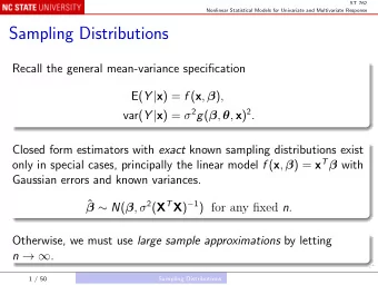
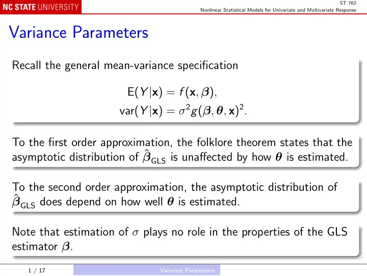
ST 762 Nonlinear Statistical Models for Univariate and Multivariate Response Variance Parameters Recall the general mean-variance specification E( Y | x ) = f ( x , β ) , var( Y | x ) = σ 2 g ( β , θ , x ) 2 . To the first order approximation, the folklore theorem states that the asymptotic distribution of ˆ β GLS is unaffected by how θ is estimated. To the second order approximation, the asymptotic distribution of ˆ β GLS does depend on how well θ is estimated. Note that estimation of σ plays no role in the properties of the GLS estimator β . 1 / 17 Variance Parameters

ST 762 Nonlinear Statistical Models for Univariate and Multivariate Response Transformed residuals Define ǫ j = Y j − f ( x j , β 0 ) σ 0 g ( β 0 , θ 0 , x j ) . Without further assumptions, E ( ǫ j | x j ) = 0 , � x j ǫ 2 � � � var ( ǫ j | x j ) = E = 1 . j We explore estimating σ based on | ǫ j | λ for various λ . 2 / 17 Variance Parameters

ST 762 Nonlinear Statistical Models for Univariate and Multivariate Response Recall key assumption The relevant moments of ǫ j are not dependent on x j and are constant for all j : E ( | ǫ j | λ | x j ) = E ( | ǫ j | λ ) = constant ∀ j , E ( | ǫ j | 2 λ | x j ) = E ( | ǫ j | 2 λ ) = constant ∀ j . For λ = 2, the first requirement is automatically met, and similarly for λ = 1 the second requirement is automatically met. 3 / 17 Variance Parameters

ST 762 Nonlinear Statistical Models for Univariate and Multivariate Response More general forms of estimating equations for θ Define η by e λη = σ λ E � | ǫ j | λ � . Identify | Y j − f ( x j , β ) | λ as the “response”. For λ = 2, η = log σ and η is simply a reparameterization; but for other λ it depends on the distribution of ǫ j : η = log σ + 1 � � | ǫ j | λ �� λ log E 4 / 17 Variance Parameters

ST 762 Nonlinear Statistical Models for Univariate and Multivariate Response Then θ and η may be estimated by solving the joint estimating equations λ � λ   � �� � � x j , ˆ − e λη g ˆ � Y j − f β , θ , x j n β � �   � λ   � � � � � ˆ ˆ g β , θ , x j β , θ , x j τ θ � 2 λ � ˆ  g β , θ , x j  j =1   = 0 where ˆ β is held fixed. T , ˆ η ) T for different We shall study the large sample distribution of (ˆ θ choices of λ . 5 / 17 Variance Parameters

ST 762 Nonlinear Statistical Models for Univariate and Multivariate Response Consistency This is an unbiased M-estimating equation, as long as ˆ β is a consistent estimator for β 0 , which we will assume. Then ˆ θ and ˆ η are consistent estimators of θ 0 and η 0 . Also note that applying the usual M-estimator argument to deduce T , ˆ η ) T requires the summand in the estimating the properties of (ˆ θ equations to be differentiable with respect to θ , η , and ˆ β . This is not always true, e.g., when λ = 1. 6 / 17 Variance Parameters

ST 762 Nonlinear Statistical Models for Univariate and Multivariate Response Asymptotic distribution for λ = 2 Complicated, depends on: whether ˆ β is based on linear or quadratic estimating equations; excess kurtosis. Simplifies if either σ 0 → 0; g ( · ) does not depend on β . Then √ n � � 0 , 2 + κ � � L ˆ θ − θ 0 − → N Λ θ . 4 7 / 17 Variance Parameters

ST 762 Nonlinear Statistical Models for Univariate and Multivariate Response Asymptotic distribution for λ = 1 Complicated, with an additional technical difficulty because of non-differentiability of | x | Simplifies if either σ 0 → 0; g ( · ) does not depend on β , and ǫ j | x j has a symmetric distribution. Then √ n � � ˆ L θ − θ 0 − → N ( 0 , c 1 Λ θ ) where c 1 = var ( | ǫ j || x j ) E ( | ǫ j || x j ) 2 . 8 / 17 Variance Parameters

ST 762 Nonlinear Statistical Models for Univariate and Multivariate Response Asymptotic distribution for general λ Equally complicated, and same technical difficulty because of non-differentiability. Simplifies if ǫ j | x j has a symmetric distribution with common absolute moments up to power 2 λ , and either σ 0 → 0; g ( · ) does not depend on β . Then √ n � � ˆ L θ − θ 0 − → N ( 0 , c λ Λ θ ) . 9 / 17 Variance Parameters

ST 762 Nonlinear Statistical Models for Univariate and Multivariate Response Here, � | ǫ j | λ � � var � x j � = � 2 , λ � = 0 , c λ � | ǫ j | λ � λ 2 E � x j � log | ǫ j | 2 � � � var � x j � = , λ = 0 . 4 So one can compare the asymptotic efficiency of the two competing methods by comparing c λ 1 and c λ 2 . 10 / 17 Variance Parameters

ST 762 Nonlinear Statistical Models for Univariate and Multivariate Response Asymptotic efficiency relative to λ = 2: c 2 / c λ Assume ǫ j is N (0 , 1) contaminated with fraction α of N (0 , 9); i.e., (1 − α ) × N (0 , 1) + α × N (0 , 9). λ = 2 λ = 1 λ = 1 α λ = 1 λ = 0 3 2 3 0.000 0.876 0.772 0.693 0.606 0.405 0.001 0.948 0.841 0.756 0.662 0.440 0.002 1.016 0.906 0.816 0.715 0.480 0.010 1.439 1.334 1.216 1.075 0.720 0.050 2.035 2.100 1.996 1.823 1.220 λ = 1 performs better than λ = 2 even for tiny levels of contamination (2 × 10 − 3 , or 2 observations per thousand). 11 / 17 Variance Parameters

ST 762 Nonlinear Statistical Models for Univariate and Multivariate Response Assume ǫ j is t -distributed with ν degrees of freedom. To match the excess kurtosis in the contaminated normal table, use ν = ∞ , 35 . 78 , 20 . 16 , 7 . 68 , 5 . 29. λ = 2 λ = 1 λ = 1 ν λ = 1 λ = 0 3 2 3 ∞ 0.876 0.765 0.693 0.610 0.405 35.78 0.921 0.813 0.741 0.655 0.439 20.16 0.965 0.861 0.787 0.698 0.471 7.68 1.270 1.191 1.111 1.002 0.695 5.29 2.016 1.994 1.897 1.739 1.234 λ = 1 performs better than λ = 2 for ν < 16. 12 / 17 Variance Parameters

ST 762 Nonlinear Statistical Models for Univariate and Multivariate Response Bottom line Asymptotic distributions of ˆ θ are complicated in general. The “small σ 0 ” simplification is quite useful and also relevant in practice. Using λ = 1 has good relative efficiency and requires estimating only E ( | ǫ j || x j ), which is not difficult. 13 / 17 Variance Parameters

ST 762 Nonlinear Statistical Models for Univariate and Multivariate Response In some circumstances, estimation of variance parameters is of critical importance. Two common such situations are prediction and calibration . Prediction Find Y given x Y 0 = f ( x 0 , ˆ ˆ β ) Calibration Find x given Y x 0 = f − 1 ( Y 0 , ˆ ˆ β ) 14 / 17 Variance Parameters

ST 762 Nonlinear Statistical Models for Univariate and Multivariate Response Variance of prediction Y 0 − ˆ Y 0 = Y 0 − f ( x 0 , ˆ β ) � � ˆ ≈ Y 0 − f ( x 0 , β 0 ) − f T β ( x 0 , β 0 ) β − β 0 15 / 17 Variance Parameters

ST 762 Nonlinear Statistical Models for Univariate and Multivariate Response Since ˆ β depends only on the training data, it is independent of Y 0 , and thus var( Y 0 − ˆ Y 0 ) ≈ var { Y 0 − f ( x 0 , β 0 ) } + f β ( x 0 , β 0 ) T var(ˆ β − β 0 ) f β ( x 0 , β 0 ) = σ 2 0 g ( x 0 , β 0 , θ 0 ) 2 0 f β ( x 0 , β 0 ) T var { n 1 / 2 (ˆ + n − 1 σ 2 β − β 0 ) } f β ( x 0 , β 0 ) ≈ σ 2 0 g ( x 0 , β 0 , θ 0 ) 2 0 f β ( x 0 , β 0 ) T { n − 1 ˆ + σ 2 Σ } f β ( x 0 , β 0 ) . 16 / 17 Variance Parameters

ST 762 Nonlinear Statistical Models for Univariate and Multivariate Response The first term in the variance reflects the uncertainty due to variation in Y 0 , and regardless of how much data are collected, the inherent variation in the response will always be there. The second term reflects uncertainty due to fitting the model to the training data, and it diminishes as more data are collected and used to fit the model. The first term dominates the second term, as the second term is O ( n − 1 ). So the predominant source of error in prediction is that due to inherent variation in the response. One can do Wald type inference for prediction based on this formula. The result for calibration is similar. 17 / 17 Variance Parameters