Defining Efficiency CSE 421: Intro Algorithms Runs fast on typical - - PowerPoint PPT Presentation

1

1

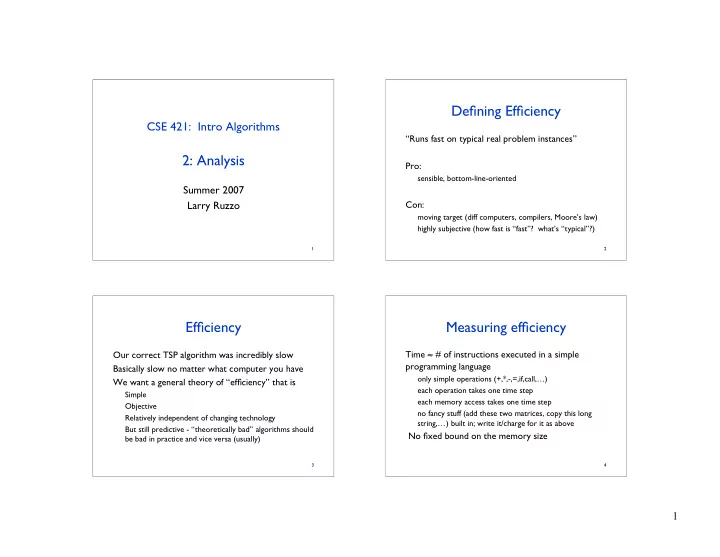
CSE 421: Intro Algorithms

2: Analysis

Summer 2007 Larry Ruzzo

2

Defining Efficiency

“Runs fast on typical real problem instances” Pro:

sensible, bottom-line-oriented

Con:

moving target (diff computers, compilers, Moore’s law) highly subjective (how fast is “fast”? what’s “typical”?)

3

Efficiency

Our correct TSP algorithm was incredibly slow Basically slow no matter what computer you have We want a general theory of “efficiency” that is

Simple Objective Relatively independent of changing technology But still predictive - “theoretically bad” algorithms should be bad in practice and vice versa (usually)

4

Measuring efficiency

Time ≈ # of instructions executed in a simple programming language

• nly simple operations (+,*,-,=,if,call,…)

each operation takes one time step each memory access takes one time step no fancy stuff (add these two matrices, copy this long string,…) built in; write it/charge for it as above

No fixed bound on the memory size

2

5

We left out things but...

Things we’ve dropped

memory hierarchy

disk, caches, registers have many orders of magnitude differences in access time

not all instructions take the same time in practice different computers have different primitive instructions

However,

the RAM model is useful for designing algorithms and measuring their efficiency

• ne can usually tune implementations so that the

hierarchy etc. is not a huge factor

6

T n

Complexity analysis

Problem size n

Worst-case complexity: max # steps algorithm takes on any input of size n Best-case complexity: min # steps algorithm takes on any input of size n Average-case complexity: avg # steps algorithm takes on inputs of size n

7

Pros and cons:

Best-case

unrealistic oversell

Average-case

• ver what probability distribution? (different people may

have different “average” problems) analysis often hard

Worst-case

a fast algorithm has a comforting guarantee maybe too pessimistic

8

Why Worst-Case Analysis?

Appropriate for time-critical applications, e.g. avionics Unlike Average-Case, no debate about what the right definition is

If worst >> average, then (a) alg is doing something pretty subtle, & (b) are hard instances really that rare?

Analysis often easier Result is often representative of "typical" problem instances Of course there are exceptions…

3

9

General Goals

Characterize growth rate of (worst-case) run time as a function of problem size, up to a constant factor Why not try to be more precise?

Technological variations (computer, compiler, OS, …) easily 10x or more Being more precise is a ton of work A key question is “scale up”: if I can afford to do it today, how much longer will it take when my business problems are twice as large? (E.g. today: cn2, next year: c(2n)2 = 4cn2 : 4 x longer.)

10

Complexity

The complexity of an algorithm associates a number T(n), the worst-case time the algorithm takes, with each problem size n. Mathematically,

T: N+ → R+ that is T is a function that maps positive integers (giving problem sizes) to positive real numbers (giving number

• f steps).

11

Problem size Time T(n)

Complexity

12

Problem size Time T(n) n log2n 2n log2n

Complexity

4

13

O-notation etc

Given two functions f and g:N→R

f(n) is O(g(n)) iff there is a constant c>0 so that f(n) is eventually always ≤ c g(n) f(n) is Ω (g(n)) iff there is a constant c>0 so that f(n) is eventually always ≥ c g(n) f(n) is Θ (g(n)) iff there is are constants c1, c2>0 so that eventually always c1g(n) ≤ f(n) ≤ c2g(n)

14

Examples

10n2-16n+100 is O(n2) also O(n3)

10n2-16n+100 ≤ 11n2 for all n ≥ 10

10n2-16n+100 is Ω (n2) also Ω (n)

10n2-16n+100 ≥ 9n2 for all n ≥16 Therefore also 10n2-16n+100 is Θ (n2)

10n2-16n+100 is not O(n) also not Ω (n3)

15

Properties

Transitivity.

If f = O(g) and g = O(h) then f = O(h). If f = Ω(g) and g = Ω(h) then f = Ω(h). If f = Θ(g) and g = Θ(h) then f = Θ(h).

Additivity.

If f = O(h) and g = O(h) then f + g = O(h). If f = Ω(h) and g = Ω(h) then f + g = Ω(h). If f = Θ(h) and g = O(h) then f + g = Θ(h).

16

2 + 2 is 4 2n2 + 5 n is O(n3) 2 + 2 = 4 2n2 + 5 n = O(n3) 4 = 2 + 2 O(n3) = 2n2 + 5 n All dogs are mammals All mammals are dogs Bottom line:

OK to put big-O in R.H.S. of equality, but not left. [Better, but uncommon, notation: T(n) ∈ O(f(n)).]

“One-Way Equalities”

5

17

Working with O-Ω-Θ notation

Claim: For any a, and any b>0, (n+a)b is Θ(nb)

(n+a)b ≤ (2n)b for n ≥ |a| = 2bnb = cnb for c = 2b so (n+a)b is O(nb) (n+a)b ≥ (n/2)b for n ≥ 2|a| (even if a <0) = 2-bnb = c’n for c’ = 2-b so (n+a)b is Ω (nb)

18

loga b = x means ax = b aloga b = b (aloga b)logb n = blogb n = n (loga b)(logb n) = loga n clogb n = loga n for the constant c = loga b So : logb n = (loga n) = (logn)

Working with O-Ω-Θ notation

Claim: For any a, b>1 logan is Θ (logbn)

19

f (n) = n2, n even n, n odd

• f(n) ≠ Θ(na) for any a.

Fortunately, such nasty cases are rare

f(n log n) ≠ Θ(na) for any a, either, but at least it’s simpler.

Big-Theta, etc. not always “nice”

20

Insertion Sort:

Ω(n2) (worst case) O(n) (best case)

A Possible Misunderstanding?

We have looked at

type of complexity analysis

worst-, best-, average-case

types of function bounds

O, Ω, Θ

These two considerations are independent of each

• ther
• ne can do any type of function bound with any type of

complexity analysis - measuring different things with same yardstick

6

21

log grows slower than every polynomial

Asymptotic Bounds for Some Common Functions

Polynomials: a0 + a1n + … + adnd is Θ(nd) if ad > 0 Logarithms: O(loga n) = O(logb n) for any constants a,b > 0 Logarithms: For all x > 0, log n = O(nx)

22

every exponential grows faster than every polynomial

Asymptotic Bounds for Some Common Functions

Exponentials. For all r > 1 and all d > 0, nd = O(rn).

n100 1.01n

23

Polynomial time

Running time is O(nd) for some constant d independent of the input size n.

24

Why It Matters

7

25

Geek-speak Faux Pas du Jour

“Any comparison-based sorting algorithm requires at least O(n log n) comparisons.”

Statement doesn't "type-check." Use Ω for lower bounds.

26

Domination

f(n) is o(g(n)) iff limn→∞ f(n)/g(n)=0

that is g(n) dominates f(n)

If a ≤ b then na is O(nb) If a < b then na is o(nb) Note: if f(n) is Θ (g(n)) then it cannot be o(g(n))

27

limn n2 n3 = limn 1 n = 0 limn n3 en = limn 3n2 en = limn 6n en = limn 6 en = 0

Working with little-o

n2 = o(n3) [Use algebra]: n3 = o(en) [Use L’Hospital’s rule 3 times]:

28

Summary

Typical initial goal for algorithm analysis is to find a

reasonably tight

i.e., Θ if possible

asymptotic

i.e., O or Θ

bound on

usually upper bound

worst case running time as a function of problem size

This is rarely the last word, but often helps separate good algorithms from blatantly poor ones - so you can concentrate on the good ones!