Sampling Distributions Recall the general mean-variance - PowerPoint PPT Presentation

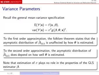
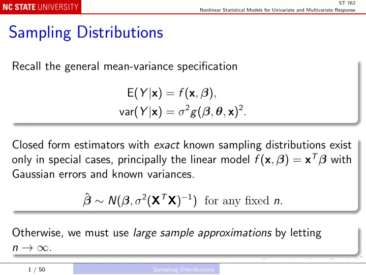
ST 762 Nonlinear Statistical Models for Univariate and Multivariate Response Sampling Distributions Recall the general mean-variance specification E( Y | x ) = f ( x , β ) , var( Y | x ) = σ 2 g ( β , θ , x ) 2 . Closed form estimators with exact known sampling distributions exist only in special cases, principally the linear model f ( x , β ) = x T β with Gaussian errors and known variances. ˆ β ∼ N ( β , σ 2 ( X T X ) − 1 ) for any fixed n . Otherwise, we must use large sample approximations by letting n → ∞ . 1 / 50 Sampling Distributions

ST 762 Nonlinear Statistical Models for Univariate and Multivariate Response Issues we aim to address Analogs of the “unbiasedness” and “minimum variance” properties. Large sample approximations that do not depend on specific distributions for the errors. Consequences of mis-specification of the variances. Tradeoffs between linear and quadratic estimating equations for β , the effect of knowing θ versus the need to estimate it. 2 / 50 Sampling Distributions

ST 762 Nonlinear Statistical Models for Univariate and Multivariate Response Fundamental concepts Asymptotic distribution. Asymptotic relative efficiency. Disclaimer A casual treatment. 3 / 50 Sampling Distributions

ST 762 Nonlinear Statistical Models for Univariate and Multivariate Response Review of Large Sample Tools a.s. Definition: almost sure convergence : Y n − → Y iff � � P n →∞ Y n = Y lim = 1 . p Definition: convergence in probability : Y n − → Y iff ∀ δ > 0, n →∞ P( | Y n − Y | < δ ) = 1 . lim p a.s. Y n − → Y ⇒ Y n − → Y but not conversely. 4 / 50 Sampling Distributions

ST 762 Nonlinear Statistical Models for Univariate and Multivariate Response If h ( · ) is continuous, then a.s. a.s. − → Y ⇒ h ( Y n ) − → h ( Y ) Y n p p − → Y ⇒ h ( Y n ) − → h ( Y ) Y n 5 / 50 Sampling Distributions

ST 762 Nonlinear Statistical Models for Univariate and Multivariate Response Terminology If ˆ η n is an estimator from a sample of size n and η 0 is the true value of the parameter, then we have two definitions of consistency: a.s. Strong consistency : ˆ η n − → η 0 ; p Weak consistency : ˆ η n − → η 0 . Interpretation Weak consistency: if the sample size n is sufficiently large, the probability is small that ˆ η n assumes a value outside an arbitrarily small neighborhood of η 0 ; i.e., for n large enough, the probability that η n will wander away is small. ˆ 6 / 50 Sampling Distributions

ST 762 Nonlinear Statistical Models for Univariate and Multivariate Response Order in probability – O p n − k || Y n || < M ǫ � � P > 1 − ǫ, for all n > n ǫ . Here � · � denotes some appropriate norm to measure magnitude of Y n . Notation: Y n = O p ( n k ); “Big” O p . 7 / 50 Sampling Distributions

ST 762 Nonlinear Statistical Models for Univariate and Multivariate Response Remarks on O p If k = 0, Y n = O p (1). Practically this says that, as n gets large, Y n does not become negligible, nor does it “blow up.” Instead, it is “nicely behaved.” If k = − 1 / 2, Y n = O p ( n − 1 / 2 ). As n → ∞ , n − 1 / 2 → 0, so Y n itself “approaches” (converges in probability to) zero at the same “rate” as n − 1 / 2 . 8 / 50 Sampling Distributions

ST 762 Nonlinear Statistical Models for Univariate and Multivariate Response Order in probability – o p p n − k Y n − → 0 , as n → ∞ . Notation: Y n = o p ( n k ); “Little” o p . 9 / 50 Sampling Distributions

ST 762 Nonlinear Statistical Models for Univariate and Multivariate Response Remarks on o p If k = − 1 / 2, Y n = o p ( n − 1 / 2 ). As n → ∞ , n − 1 / 2 → 0, so Y n itself “approaches” (converges in probability to) zero at a faster “rate” than n − 1 / 2 . 10 / 50 Sampling Distributions

ST 762 Nonlinear Statistical Models for Univariate and Multivariate Response Properties If X n = o p ( n k 1 ) and Y n = o p ( n k 2 ), then X n Y n = o p ( n k 1 + k 2 ) If X n = o p ( n k 1 ) and Y n = O p ( n k 2 ), then X n Y n = o p ( n k 1 + k 2 ) Note that Y n = o p ( n ) ⇒ Y n = O p ( n ), so the second property implies the first. 11 / 50 Sampling Distributions

ST 762 Nonlinear Statistical Models for Univariate and Multivariate Response Convergence in distribution L Definition: convergence in distribution (or law): Y n − → Y iff for each continuity point y of F Y ( · ), n →∞ F Y n ( y ) = F Y ( y ) . lim p L Note: Y n − → Y ⇒ Y n − → Y but, in general, not conversely. L Special (and trivial) case: if Y n − → y where y is a constant, then p − → y . Y n Practical interpretation If we are interested in probability and distributional statements about Y n , we may approximate these with statements about Y . 12 / 50 Sampling Distributions

ST 762 Nonlinear Statistical Models for Univariate and Multivariate Response Asymptotic normality If we can find sequences { a n } and { c n > 0 } such that L c n ( Y n − a n ) − → N (0 , 1) we say that Y n is asymptotically normal with asymptotic mean a n and asymptotic variance c − 2 n . We write � � a n , 1 · Y n ∼ N . c 2 n 13 / 50 Sampling Distributions

ST 762 Nonlinear Statistical Models for Univariate and Multivariate Response Central Limit Theorem Z j are independent with E( Z j ) = µ j , var( Z j ) = Σ j . The variance matrices satisfy 1 lim n ( Σ 1 + Σ 2 + · · · + Σ n ) = Σ . n →∞ The tails of the distributions of Z j satisfy the Lindeberg condition: ∀ ǫ > 0, n 1 � � || z − µ j || 2 dF j ( z ) → 0 as n → ∞ . || Z j − µ j ||≥ ǫ √ n n j =1 14 / 50 Sampling Distributions

ST 762 Nonlinear Statistical Models for Univariate and Multivariate Response Then n 1 L � � � √ n Z j − µ j − → N ( 0 , Σ ) . j =1 In the language of asymptotic normality: if n Z n = 1 ¯ � Z j n j =1 and n µ n = 1 � ¯ µ j , n j =1 then � � µ n , 1 · ¯ Z n ∼ N ¯ n Σ . 15 / 50 Sampling Distributions

ST 762 Nonlinear Statistical Models for Univariate and Multivariate Response More general CLT If we also write n Σ n = 1 ¯ � Σ j , n j =1 the variance matrix condition can be written ¯ lim Σ n = Σ . n →∞ A more general CLT does not require this convergence: � � µ n , 1 · ¯ ¯ Z n ∼ N ¯ Σ n . n 16 / 50 Sampling Distributions

ST 762 Nonlinear Statistical Models for Univariate and Multivariate Response The Lindeberg condition becomes: ∀ ǫ > 0, n 1 � 1 {|| Z j − µ j ||≥ ǫ √ n λ n } || Z j − µ j || 2 � � E → 0 as n → ∞ , n λ n j =1 where λ n is the smallest eigenvalue of ¯ Σ n . Under only this modified Lindeberg condition, � µ n , 1 � · ¯ ¯ Z n ∼ N ¯ Σ n . n 17 / 50 Sampling Distributions

ST 762 Nonlinear Statistical Models for Univariate and Multivariate Response In terms of convergence in distribution: L � ¯ � C n Z n − ¯ − → N ( 0 , I ) µ n n ¯ where C n is any inverse square root of 1 Σ n : � 1 � ¯ C T C n Σ n n = I . n 18 / 50 Sampling Distributions

ST 762 Nonlinear Statistical Models for Univariate and Multivariate Response Slutsky’s Theorem p L If Y n − → Y and V n − → c , a constant, then: L Y n + V n − → Y + c L − → cY Y n V n and, if c � = 0, L Y n / V n − → Y / c . 19 / 50 Sampling Distributions

ST 762 Nonlinear Statistical Models for Univariate and Multivariate Response Multivariate version L p If Y n − → Y and V n − → C , a constant matrix, then: L Y n + V n − → Y + C L V n Y n − → CY and, if C is nonsingular, L V − 1 → C − 1 Y . n Y n − 20 / 50 Sampling Distributions

ST 762 Nonlinear Statistical Models for Univariate and Multivariate Response Weak Law of Large Numbers { Z j } are uncorrelated and { a j } are constants. If � � n n 1 = 1 � � a 2 var j var ( Z j ) → 0 as n → ∞ , a j Z j n 2 n j =1 j =1 then n n 1 a j Z j − 1 p � � a j E ( Z j ) − → 0 . n n j =1 j =1 p Furthermore, if n − 1 � n j =1 a j E ( Z j ) → c , then n − 1 � n − → c . j =1 a j Z j The condition is satisfied if n − 1 � n j =1 a 2 j var( Z j ) → c , which is a similar requirement to the CLT. 21 / 50 Sampling Distributions

ST 762 Nonlinear Statistical Models for Univariate and Multivariate Response How do we use all these results? Suppose that some estimator ˆ η satisfies √ n (ˆ η − η 0 ) = A − 1 n C n + o p (1) , where: p A n satisfies the WLLN, and A n − → C , a constant matrix; C n satisfies the CLT, and is asymptotically normal with zero mean. · Then ˆ ∼ N ( η 0 , Σ n ) for some asymptotic variance matrix Σ n , η typically of the form n − 1 Σ . 22 / 50 Sampling Distributions

ST 762 Nonlinear Statistical Models for Univariate and Multivariate Response Comparing estimators η (1) and ˆ η (2) are both asymptotically normal with Suppose that ˆ asymptotic mean η 0 , but with different asymptotic variance matrices n − 1 Σ (1) and n − 1 Σ (2) . Which should we prefer? In the univariate case, the one with the smaller asymptotic variance. 23 / 50 Sampling Distributions