
Variable Selection and Model Choice in Survival Models with - PowerPoint PPT Presentation
Variable Selection and Model Choice in Survival Models with Time-Varying Effects Boosting Survival Models Benjamin Hofner 1 Department of Medical Informatics, Biometry and Epidemiology (IMBE) Friedrich-Alexander-Universit at Erlangen-N
Variable Selection and Model Choice in Survival Models with Time-Varying Effects Boosting Survival Models Benjamin Hofner 1 Department of Medical Informatics, Biometry and Epidemiology (IMBE) Friedrich-Alexander-Universit¨ at Erlangen-N¨ urnberg joint work with Thomas Kneib and Torsten Hothorn Department of Statistics Ludwig-Maximilians-Universit¨ at M¨ unchen useR! 2008 1 benjamin.hofner@imbe.med.uni-erlangen.de
Introduction Technical Preparations Cox flex Boost Summary / Outlook References Introduction Cox PH model: λ i ( t ) = λ ( t , x i ) = λ 0 ( t ) exp( x ′ i β ) with λ i ( t ) hazard rate of observation i [ i = 1 , . . . , n ] λ 0 ( t ) baseline hazard rate x i vector of covariates for observation i [ i = 1 , . . . , n ] β vector of regression coefficients Problem: restrictive model, not allowing for non-proportional hazards (e.g., time-varying effects) non-linear effects
Introduction Technical Preparations Cox flex Boost Summary / Outlook References Additive Hazard Regression Generalisation: Additive Hazard Regression (Kneib & Fahrmeir, 2007) λ i ( t ) = exp( η i ( t )) with J � η i ( t ) = f j ( x i ( t )) , j =1 generic representation of covariate effects f j ( x i ) a) linear effects: f j ( x i ( t )) = f linear (˜ x i ) = ˜ x i β b) smooth effects: f j ( x i ( t )) = f smooth (˜ x i ) c) time-varying effects: f j ( x i ( t )) = f smooth ( t ) · ˜ x i where ˜ x i ∈ x i ( t ). Note: c) includes log-baseline for ˜ x i ≡ 1
Introduction Technical Preparations Cox flex Boost Summary / Outlook References P-Splines flexible terms can be represented using P-splines (Eilers & Marx, 1996) model term ( x can be either ˜ x i or t ): � M f j ( x ) = β jm B jm ( x ) ( j = 1 , . . . , J ) m =1 penalty: � κ j β j ′ K β j cases b),c) pen j ( β j ) = 0 case a) with K = D ′ D (i.e., cross product of difference matrix D ) � 1 � − 2 1 . . . e . g . D = 0 1 − 2 1 . . . κ j smoothing parameter (larger κ j ⇒ more penalization ⇒ smoother fit)
Introduction Technical Preparations Cox flex Boost Summary / Outlook References Inference Penalized Likelihood Criterion: (NB: this is the full log-likelihood) � � t i � n J � � L pen ( β ) = δ i η i ( t i ) − exp( η i ( t )) dt − pen j ( β j ) 0 i =1 j =0 T i true survival time C i censoring time t i = min( T i , C i ) observed survival time (right censoring) δ i = 1 ( T i ≤ C i ) indicator for non-censoring Problem: Estimation and in particular model choice
Introduction Technical Preparations Cox flex Boost Summary / Outlook References Cox flex Boost Aim: Maximization of a (potentially) high-dimensional log-likelihood with different modeling alternatives Thus, we use: Iterative algorithm Likelihood-based boosting algorithm Component-wise base-learners Therefore: Use one base-learner g j ( · ) for each covariate (or each model component) [ j ∈ { 1 , . . . , J } ] Component-Wise Boosting as a means of estimation and variable selection combined with model choice.
Introduction Technical Preparations Cox flex Boost Summary / Outlook References Cox flex Boost Aim: Maximization of a (potentially) high-dimensional log-likelihood with different modeling alternatives Thus, we use: Iterative algorithm Likelihood-based boosting algorithm Component-wise base-learners Therefore: Use one base-learner g j ( · ) for each covariate (or each model component) [ j ∈ { 1 , . . . , J } ] Component-Wise Boosting as a means of estimation and variable selection combined with model choice.
Introduction Technical Preparations Cox flex Boost Summary / Outlook References Cox flex Boost Aim: Maximization of a (potentially) high-dimensional log-likelihood with different modeling alternatives Thus, we use: Iterative algorithm Likelihood-based boosting algorithm Component-wise base-learners Therefore: Use one base-learner g j ( · ) for each covariate (or each model component) [ j ∈ { 1 , . . . , J } ] Component-Wise Boosting as a means of estimation and variable selection combined with model choice.
Introduction Technical Preparations Cox flex Boost Summary / Outlook References Cox flex Boost Algorithm (i) Initialization: Iteration index m := 0. Function estimates (for all j ∈ { 1 , . . . , J } ): ˆ f [0] ( · ) ≡ 0 j Offset (MLE for constant log hazard): �� n � i =1 δ i η [0] ( · ) ≡ log ˆ � n i =1 t i
Introduction Technical Preparations Cox flex Boost Summary / Outlook References (ii) Estimation: m := m + 1. Fit all (linear/P-spline) base-learners separately g j = g j ( · ; ˆ ˆ β j ) , ∀ j ∈ { 1 , . . . , J } , by penalized MLE, i.e., ˆ L [ m ] β j = arg max j , pen ( β ) β with the penalized log-likelihood ( analogously as above ) � � n L [ m ] η [ m − 1] j , pen ( β ) = δ i · (ˆ + g j ( x i ( t i ); β )) i i =1 � � t i � � η [ m − 1] ( ˜ t ) + g j ( x i ( ˜ d ˜ − exp ˆ t ); β ) t − pen j ( β ) , i 0 with the additive predictor η i split η [ m − 1] into the estimate from previous iteration ˆ i and the current base-learner g j ( · ; β )
Introduction Technical Preparations Cox flex Boost Summary / Outlook References (iii) Selection: Choose base-learner ˆ g j ∗ with j ∗ = arg j ∈{ 1 ,..., J } L [ m ] j , unpen (ˆ max β j ) (iv) Update: Function estimates (for all j ∈ { 1 , . . . , J } ): � ˆ f [ m − 1] + ν · ˆ g j j = j ∗ f [ m ] ˆ j = f [ m − 1] ˆ j j � = j ∗ j Additive predictor (= fit): η [ m ] = ˆ η [ m − 1] + ν · ˆ ˆ g j ∗ with step-length ν ∈ (0 , 1] (here: ν = 0 . 1) (v) Stopping rule: Continue iterating steps (ii) to (iv) until m = m stop
Introduction Technical Preparations Cox flex Boost Summary / Outlook References Some Aspects of Cox flex Boost Estimation full penalized MLE · ν (step-length) based on unpenalized log-likelihood L [ m ] Selection j , unpen specified by (initial) degrees of freedom, i.e., df j = � Base-Learners df j Likelihood-based boosting (in general): See, e.g., Tutz and Binder (2006) Above aspects in Cox flex Boost: See, e.g., model based boosting (B¨ uhlmann & Hothorn, 2007)
Introduction Technical Preparations Cox flex Boost Summary / Outlook References Degrees of Freedom Specifying df more intuitive than specifying smoothing parameter κ Comparable to other modeling components, e.g., linear effects Problem: Not constant over the (boosting) iterations But simulation studies showed: No big deviation from the initial df j = � df j bbs ( x 3 ) 1.0 Estimated degrees of freedom traced 0.8 over the boosting steps for the flexi- 0.6 df ( m ) ble base-learners of x 3 (in 200 repli- 0.4 cates) and initially specified degrees 0.2 of freedom (dashed line). 0.0 0 200 400 600 800 boosting iteration m
Introduction Technical Preparations Cox flex Boost Summary / Outlook References Model Choice Recall from generic representation: f j (˜ x i ) can be a a) linear effect: f j ( x i ( t )) = f linear (˜ x i ) = ˜ x i β b) smooth effect: f j ( x i ( t )) = f smooth (˜ x i ) c) time-varying effect: f j ( x i ( t )) = f smooth ( t ) · ˜ x i ⇒ We see: ˜ x i can enter the model in 3 different ways But how? Add all possibilities as base-learners to the model. Boosting can chose between the possibilities But the df must be comparable! Otherwise: more flexible base-learners are preferred
Introduction Technical Preparations Cox flex Boost Summary / Outlook References Model Choice Recall from generic representation: f j (˜ x i ) can be a a) linear effect: f j ( x i ( t )) = f linear (˜ x i ) = ˜ x i β b) smooth effect: f j ( x i ( t )) = f smooth (˜ x i ) c) time-varying effect: f j ( x i ( t )) = f smooth ( t ) · ˜ x i ⇒ We see: ˜ x i can enter the model in 3 different ways But how? Add all possibilities as base-learners to the model. Boosting can chose between the possibilities But the df must be comparable! Otherwise: more flexible base-learners are preferred
Introduction Technical Preparations Cox flex Boost Summary / Outlook References For higher order differences ( d ≥ 2): df > 1 ( κ → ∞ ) Polynomial of order d − 1 remains unpenalized Solution: Decomposition (based on Kneib, Hothorn, & Tutz, 2008) g ( x ) = β 0 + β 1 x + . . . + β d − 1 x d − 1 + g centered ( x ) � �� � � �� � unpenalized, parametric part deviation from polynomial Add unpenalized part as separate, parametric base-learners Assign df = 1 to the centered effect (and add as P-spline base-learner) Analogously for time-varying effects Technical realization (see Fahrmeir, Kneib, & Lang, 2004): decomposing the vector of regression coefficients β into ( � β unpen , � β pen ) utilizing a spectral decomposition of the penalty matrix
Introduction Technical Preparations Cox flex Boost Summary / Outlook References Early Stopping 1 Run the algorithm m stop -times (previously defined). 2 Determine new � m stop , opt ≤ m stop : ... based on out-of-bag sample (with simulations easy to use) ... based on information criterion, e.g., AIC ⇒ Prevents algorithm to stop in a local maximum (of the log-likelihood) ⇒ Early stopping prevents overfitting
Recommend


More recommend
Explore More Topics
Stay informed with curated content and fresh updates.