P -spline ANOVA-type interaction models for spatio-temporal - PowerPoint PPT Presentation
P -spline ANOVA-type interaction models for spatio-temporal smoothing Dae-Jin Lee and Mar a Durb an Universidad Carlos III de Madrid Department of Statistics IWSM Utrecht 2008 D.-J. Lee and M. Durban (UC3M) P -spline
P -spline ANOVA-type interaction models for spatio-temporal smoothing Dae-Jin Lee ⋆ and Mar´ ıa Durb´ an Universidad Carlos III de Madrid Department of Statistics IWSM Utrecht 2008 D.-J. Lee and M. Durban (UC3M) ’ P -spline ANOVA-type models’ IWSM 2008 1 / 26
Outline 1 Motivation 2 Penalized splines for Spatio-Temporal data 3 ANOVA-Type Interaction Models 4 Application to O 3 pollution in Europe 5 Conclusions D.-J. Lee and M. Durban (UC3M) ’ P -spline ANOVA-type models’ IWSM 2008 2 / 26
1. Motivation • Air pollution • Enviromental policies • Monitoring networks: ◮ European Environmental Agency ( EEA ) ◮ EMEP project (European Monitoring and Evaluation Programme) • Ozone ( O 3 ) is currently one of the air pollutants of most concern in Europe. D.-J. Lee and M. Durban (UC3M) ’ P -spline ANOVA-type models’ IWSM 2008 3 / 26
Monitoring stations across Europe ● ● ● ● ● ● ● ● ● ● ● ● ● ● ● ● ● ● ● ● ● ● ● ● ● ● ● ● ● ● ● ● ● ● ● ● ● ● ● ● ● ● ● ● −5 0 5 10 15 20 25 sample of 45 monitoring stations Monitoring station D.-J. Lee and M. Durban (UC3M) ’ P -spline ANOVA-type models’ IWSM 2008 4 / 26
O 3 time series plot for selected locations ◮ Seasonal pattern: Spain Finland 140 France UK 120 100 80 60 40 20 1999 2000 2001 2002 2003 2004 2005 time D.-J. Lee and M. Durban (UC3M) ’ P -spline ANOVA-type models’ IWSM 2008 5 / 26
O 3 level from 01 / 2004 to 12 / 2005 Play animation 20 20 20 40 40 40 60 60 60 80 80 80 100 100 100 120 120 120 D.-J. Lee and M. Durban (UC3M) ’ P -spline ANOVA-type models’ IWSM 2008 6 / 26
1. Motivation ◮ Spatio-temporal data • Response variable, y ijt ◮ measured over geographical locations , s = ( x i , x j ), with i , j = 1 , .., n ◮ and over time periods , x t , for t = 1 , ...., T • ISSUE: huge amount of data available ◮ e.g. : Environmental data, epidemiologic studies, disease mapping applications, ... • Smoothing techniques: ◮ Study spatial and temporal trends. ◮ Space and time interactions. ◮ “Penalized Splines” ( Eilers and Marx, 1996 ). D.-J. Lee and M. Durban (UC3M) ’ P -spline ANOVA-type models’ IWSM 2008 7 / 26
2. Penalized splines ◮ “The flexible smoother” • Methodology: ◮ Given the data ( x i , y i ), i = 1 , ..., n . ◮ Fit a sum of local basis functions : f ( x i ) = B θ ◮ Minimize the Penalized Sum of Squares : � y i − f ( x i ) � 2 + Penalty ◮ The Penalty controls the smoothness of the fit. � Smoothing parameter : λ � Apply a discrete penalty over coefficients θ , e.g. in 1 d : P = λ D ′ D where D is a difference matrix acting on θ . D.-J. Lee and M. Durban (UC3M) ’ P -spline ANOVA-type models’ IWSM 2008 8 / 26
2. Penalized splines ◮ “The flexible smoother” • For array data ( Currie et al., 2006 ): ◮ Generalized Linear Array Methods (GLAM): f ( x 1 , ..., x d ) = B θ ◮ where B is the Kronecker product of d B -splines basis: B = B 1 ⊗ B 2 ⊗ .... ⊗ B d ◮ Efficient Algorithms for smoothing on multidimensional grids ( e.g. mortality data, images, etc...). ◮ Easy representation as a Mixed Model: f ( x 1 , ..., x d ) = X β + Z α D.-J. Lee and M. Durban (UC3M) ’ P -spline ANOVA-type models’ IWSM 2008 9 / 26
2. Penalized splines ◮ Example of GLAM: • 3 d -case: f ( x 1 , x 2 , x 3 ) = B θ • Basis: B = B 1 ⊗ B 2 ⊗ B 3 ◮ θ can be expressed as a 3 d -array A = { θ } ijk of dim. c 1 × c 2 × c 3 θ (1 , 1 , c 3 ) θ (1 , c 2 , c 3 ) � � � � layer � � � � � � � � 1 ,..., c 3 � � � � � � columns θ (1 , 1 , 1) θ (1 , c 2 , 1) 1 ,..., c 2 θ ( c 1 , 1 , c 3 ) θ ( c 1 , c 2 , c 3 ) rows 1 ,..., c 1 � � � � � � � � � θ ( c 1 , 1 , 1) θ ( c 1 , c 2 , 1) D.-J. Lee and M. Durban (UC3M) ’ P -spline ANOVA-type models’ IWSM 2008 10 / 26
• 3 d Penalty matrix: ◮ Set penalties over the 3 d -array A : P = λ 1 D ′ + λ 2 I c 1 ⊗ D ′ + λ t I c 1 ⊗ I c 2 ⊗ D ′ 1 D 1 ⊗ I c 2 ⊗ I c 3 2 D 2 ⊗ I c 3 t D t � �� � � �� � � �� � row-wise column-wise layer-wise ◮ For spatio-temporal data : f ( longitude , latitude , time ) � �� � Space � Spatial anisotropy ( λ 1 � = λ 2 ), different amount of smoothing for latitude and longitude. � Temporal smoothing ( λ t ) � Space-time interaction . � However spatial data are not over a regular grid . D.-J. Lee and M. Durban (UC3M) ’ P -spline ANOVA-type models’ IWSM 2008 11 / 26
2. Penalized splines ◮ Scattered data smoothing • For scattered data, Eilers et al. (2006) , propose: ◮ “Row-wise Kronecker” product or Box-Product of B -spline basis. Def. Box-Product: B 1 � B 2 = ( B 1 ⊗ 1 ′ c 2 ) ⊙ ( 1 ′ c 1 ⊗ B 2 ) where ⊙ is the element-wise product. ◮ We propose the use of � for spatial data: � Although spatial data are not over a grid, � the coefficients θ can be expressed in array form. � Choose a moderate number of knots to cover the spatial domain. D.-J. Lee and M. Durban (UC3M) ’ P -spline ANOVA-type models’ IWSM 2008 12 / 26
2. Penalized splines ◮ Spatio-Temporal data smoothing • For spatio-temporal data , we propose: Spatio-temporal B -splines Basis: B = B s ⊗ B t , of dim. nt × c 1 c 2 c 3 where B s ≡ is the spatial B -spline basis ( B 1 � B 2 ) and B t ≡ is the B -spline basis for time of dim. t × c 3 . • Note that: ◮ GLAM framework ◮ Mixed models ( � ) D.-J. Lee and M. Durban (UC3M) ’ P -spline ANOVA-type models’ IWSM 2008 13 / 26
2. Penalized splines ◮ Mixed Models representation • Reparameterize the basis B and coefficients θ : B θ = X β + Z α • Currie et al. (2006) , use the Singular Value Decomposition (SVD) over the Penalty P , i.e.: � � � � U ′ 0 q n D ′ D = [ U n : U s ] � U ′ Σ s • The Penalty becomes (blockdiagonal) , F = λ � Σ • Standard mixed model theory ( REML ) D.-J. Lee and M. Durban (UC3M) ’ P -spline ANOVA-type models’ IWSM 2008 14 / 26
3. ANOVA-Type Interaction Models ◮ Smooth-ANOVA decomposition models • Chen (1993), Gu (2002): ◮ “Smoothing-Spline ANOVA” (SS-ANOVA) . ◮ Interpretation as “main effects” and “interactions” . ◮ Models of type: � y = f ( x 1 ) + f ( x 2 ) + f ( x t ) “Main/additive effects” + f ( x 1 , x 2 ) + f ( x 1 , x t ) + f ( x 2 , x t ) “2-way interactions” + f ( x 1 , x 2 , x t ) “3-way interactions” ◮ PROBLEM: basis dimension ( “curse of dimensionality” ) D.-J. Lee and M. Durban (UC3M) ’ P -spline ANOVA-type models’ IWSM 2008 15 / 26
3. ANOVA-Type Interaction Models ◮ Smooth-ANOVA decomposition models • We propose ANOVA-Type models: ◮ Computationally efficient methodology � based on low-rank P -splines and GLAM . ◮ For Spatio-temporal smoothing : � Interpretation as: main spatial and temporal effects, • spatial 2 d effects ( anisotropy) and • space-time interaction • ◮ Our approach is based on: � SVD properties and � the mixed model representation D.-J. Lee and M. Durban (UC3M) ’ P -spline ANOVA-type models’ IWSM 2008 16 / 26
• ANOVA-Type Interaction models: ◮ 3 d model: f ( x 1 , x 2 , x t ) with basis: B = B s ⊗ B t and smoothing parameters ( λ 1 , λ 2 , λ t ), can be decomposed as: f ( x 1 ) + f ( x 2 ) + f ( x t ) + f ( x 1 , x 2 ) + ... + f ( x 1 , x 2 , x t ) � Reformulate as a mixed model and expand the basis X and Z . D.-J. Lee and M. Durban (UC3M) ’ P -spline ANOVA-type models’ IWSM 2008 17 / 26
Expand X and Z Basis main effects 2-way interact. 3-way interact. X columns x 1 : x 2 : x 3 ( x 1 , x 2 ) : ( x 2 , x 3 ) : ( x 1 , x 3 ) ( x 1 , x 2 , x 3 ) ≡ Z blocks ′′ ′′ ′′ ≡ Penalty λ 1 , λ 2 , λ t and � Σ 1 , � Σ 2 , � F blockdiag Σ t ≡ D.-J. Lee and M. Durban (UC3M) ’ P -spline ANOVA-type models’ IWSM 2008 18 / 26
◮ Full-ANOVA-type model: f ( x 1 ) + f ( x 2 ) + f ( x t ) + f ( x 1 , x 2 ) + ... + f ( x 1 , x 2 , x t ) different λ ’s for each smooth f ( · ), with basis B = [ B 1 s ⊗ 1 t : B 2 s ⊗ 1 t : 1 n ⊗ B t : B s ⊗ 1 t : B s ⊗ B t ] � However now, B is NOT full column-rank ( “linear dependency” ) � Model is NOT identifiable ◮ The mixed model representation and the expansion of X and Z , allow us to identify the constraints to impose in order to maintain the identifiability of the model. ◮ In P -splines context: � constraints are applied over regression coefficients θ i , j , k D.-J. Lee and M. Durban (UC3M) ’ P -spline ANOVA-type models’ IWSM 2008 19 / 26
Equivalent as in a 3-way factorial design � main effects: � � � θ (1) θ (2) θ (3) = = = 0 t i j t i j � 2-way interactions: � � � θ (1 , 2) θ (2 , 3) θ (1 , 3) = = = 0 ij it jt i , j i , t j , t � 3-way interactions: � θ (1 , 2 , 3) = 0 ijt i , j , t D.-J. Lee and M. Durban (UC3M) ’ P -spline ANOVA-type models’ IWSM 2008 20 / 26
Recommend
More recommend
Explore More Topics
Stay informed with curated content and fresh updates.
