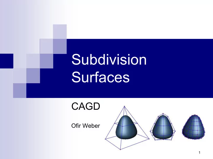
Subdivision Surfaces CAGD Ofir Weber 1 Spline Surfaces Spline - PowerPoint PPT Presentation

Subdivision Surfaces CAGD Ofir Weber 1

Spline Surfaces Spline Surfaces � Why use them? � Smooth � Good for modeling - easy to control � Compact (complex objects are represented by less numbers) � Flexibility (different tessellation-parameters produce different level-of-details from the same surface) 2

Disadvantages of Splines � Grid should be regular � Resolution is not adaptive � Problems along seams of patchwork � Not well suited for animation – deformable models � Topology is not arbitrary (Holes, trim curves) � Less easy to add “features” such as crease. 3

Subdivision Surfaces – The Alternative 4

Applications: Mainly Computer Graphics / animation 5

The basic idea ∞ 0 1 2 V V V V � In each iteration � Refine a control net (mesh) � Increases the number of vertices / faces � The mesh vertices converges to a limit surface � Each subdivision scheme has: � Rules to calculate the locations of new vertices. � A method to generate the new net topology. 6

Subdivision schemes ”Subdivision Zoo” Classification: � Catmul Clark � Mesh types: tris, quads, hex…, combination � Doo Sabin � Face / vertex split � Loop � Interpolating / Approximating � Butterfly – Nira Dyn � Smoothness � …many more � (Non)Linear � … 7

Uniform Cubic Bi-variant Tensor product B-spline Patch Splitting We can express the bicubic B-spline patch by: � = t t where S u v ( , ) UMGM V − − ⎡ ⎤ ⎡ ⎤ 1 3 3 1 P P P P 11 12 13 14 ⎢ ⎥ ⎢ ⎥ − 3 6 3 0 P P P P 1 ⎢ ⎥ ⎢ ⎥ = = ⎢ 21 22 23 24 M G ⎥ ⎢ ⎥ − 6 3 0 3 0 P P P P ⎢ 31 32 33 34 ⎥ ⎢ ⎥ ⎣ ⎦ ⎣ ⎦ 1 4 1 0 P P P P 41 42 43 44 ⎡ ⎤ = ⎣ 3 2 1 U u u u ⎦ ⎡ ⎤ = ⎣ 3 2 V v v v 1 ⎦ M - B-Spline basis matrix � G - set of control points � U,V - are the primitive basis vectors. � 8

B-Spline Splitting (cont’) We will limit our discussion to one quadrant of the patch in which 0<u,v<½ , as it is identical to the others, due to symmetry. = = This is the sub-patch where S ( u 1 v , ) u u / 2 , v v / 2 1 1 1 We can now combine the two last expressions into: = t t t S u v ( , ) USMGM S V 1 1 ⎡ ⎤ 1 0 0 0 ⎢ ⎥ 8 ⎢ ⎥ where: ⎢ ⎥ 1 0 0 0 ⎢ ⎥ = S 4 ⎢ ⎥ 1 ⎢ ⎥ 0 0 0 ⎢ ⎥ 2 ⎢ ⎥ ⎣ ⎦ 0 0 0 1 9

B-Spline Splitting (cont’) � Notice that the new patch must still be a bicubic B-spline surface and therefore must satisfy: = t t ( , ) S u v UMG M V 1 1 1 = t t t Thus it must uphold: MG M SMGM S 1 M is invertible so we can write it as: ( ) ( ) − − = = 1 t t t t G M SM G M S M H GH 1 1 1 Where ⎡ ⎤ 4 4 0 0 ⎢ ⎥ 1 6 1 0 1 ⎢ ⎥ − = = 1 H M SM ⎢ ⎥ 1 8 0 4 4 0 ⎢ ⎥ ⎣ ⎦ 0 1 6 1 10

B-Spline Splitting (cont’) And for individual points noted as qij: ( ) + + + p p p p = 11 12 21 22 q Face point: 11 4 + + ⎛ ⎞ ⎛ ⎞ q q p p + ⎜ 11 13 12 22 ⎜ ⎟ ⎟ ⎝ ⎠ ⎝ ⎠ Edge point: 2 2 = q 12 2 Vertex point: Q R p = + + 22 q 22 4 2 4 ( ) + + + q q q q = 11 13 31 33 Q 4 ( ) ( ) ( ) ( ) ⎡ ⎤ + + + + p p p p p p p p 1 = + + + 22 12 22 21 22 32 22 23 ⎢ ⎥ R 4 ⎣ 2 2 2 2 ⎦ 11

Catmull-Clark scheme ’78 Face Point m 1 ∑ = f p i m = i 1 Edge Point + + + p p f f = 1 2 1 2 e 4 Vertex Point − Q 2 R p ( n 3) = + + v n n n � Q – Average of face points − � R – Average of midpoints n n 1 1 n 2 ∑ ∑ = + + v f e p � P – old vertex i i 2 2 n n n 12 = = i 1 i 1

Keep subdividing… � After 1 iteration, Every new face is a rectangular. � Extraordinary vertices are forever. Valence is retained. � Ultimately, at the limit, the surface will be a standard bicubic B-spline surface at every point except at these “extraordinary points”, and therefore at all but extraordinary points. ( 2 ) C � Catmull & Clark did not prove or guarantee continuity at the extraordinary points but note that trials indicate this much. � Later on it was proven to be C1 13

Catmull-Clark, special rules Crease/body masks 6 1 8 8 1 2 1 2 1 8 Piecewise smooth surface 14

Catmull-Clark - Summary � Any topology – better use quad faces and vertices with valence 4 � Approximation � Generalization of cubic B-Spline � Face Split � C2 everywhere. C1 on extraordinary vertices � Linear 15

Behavior near Extraordinary Points - Doo Sabin 78’ � Extraordinary faces turns into extraordinary points after the first iteration � After that, the number of extraordinary points stays constant � The distance between extraordinary points remains, more or less ,fixed, And the number of faces between them grows with every step � Hence, we can treat each extraordinary point as an isolated phenomenon on a regular lattice 16

Matrix Form ⎡ ⎤ ⎡ ⎤ ⎡ ⎤ q Q 1 1 ⎢ ⎥ ⎢ ⎥ ⎢ ⎥ ⋅ ⋅ ⎢ ⎥ ⎢ ⎥ ⎢ ⎥ ( ) ⎢ ⋅ ⎥ ⎢ ⎥ ⎢ ⋅ ⎥ = + + + q Q R R S / 4 ⎢ ⎥ ⎢ ⎥ ⎢ ⎥ + i i i i 1 q Q ⎢ ⎥ ⎢ ⎥ ⎢ ⎥ ( ) n n = + + + ⎢ ⎥ ⎢ ⎥ ⎢ ⎥ = r q q R S / 4 r M R − i i i 1 i ⎢ ⎥ ⎢ ⎥ ⎢ ⎥ 1 1 ⋅ ⋅ ⎢ ⎥ ⎢ ⎥ ⎢ ⎥ ⎛ ⎞ q R ∑ ∑ ⎢ ⎥ ⎢ ⎥ ⎢ ⎥ ⋅ ⋅ = + + i i ⎜ ⎟ s 2 S / 4 ⎢ ⎥ ⎢ ⎥ ⎢ ⎥ ⎝ ⎠ n n ⎢ ⎥ ⎢ ⎥ ⎢ ⎥ r R i i n n ⎢ ⎥ ⎢ ⎥ ⎢ ⎥ ⎣ ⎦ ⎣ ⎦ ⎣ ⎦ s S 17

Matrix form for n=4 ⎛ ⎞ 1 1 1 1 0 0 0 0 0 ⎜ ⎟ 4 4 4 4 ⎜ ⎟ � Matrix is large ⎜ ⎟ 1 1 1 1 0 0 0 0 0 ⎜ ⎟ ⎛ ⎛ ⎞ ⎞ 4 4 4 4 q Q ⎜ ⎟ ⎜ ⎜ ⎟ ⎟ 1 1 1 1 1 1 ⎜ ⎟ ⎜ ⎜ ⎟ ⎟ 0 0 0 0 0 q Q ⎜ ⎟ ⎜ � We want to ⎜ ⎟ 4 4 4 4 ⎟ 2 2 ⎜ ⎟ ⎜ ⎜ ⎟ ⎟ 1 1 1 1 q ⎜ ⎟ ⎜ Q ⎜ ⎟ 0 0 0 0 0 ⎟ 3 ⎜ ⎟ ⎜ 3 4 4 4 4 analyze for all ⎜ ⎟ ⎟ ⎜ ⎟ ⎜ q Q ⎜ ⎟ = ⎟ 1 1 6 1 1 6 i ⎜ ⎟ ⎜ 4 0 0 0 4 ⎜ ⎟ ⎟ ⎜ 16 16 16 16 16 16 ⎟ ⎜ r R possible n ⎜ ⎟ ⎟ 1 1 ⎜ ⎟ ⎜ 1 1 1 6 1 6 ⎜ ⎟ ⎟ r R 0 0 0 ⎜ ⎟ ⎜ ⎜ 2 ⎟ 2 ⎟ 16 16 16 16 16 16 ⎜ ⎟ ⎜ r R ⎜ ⎟ ⎟ 3 ⎜ ⎟ ⎜ 3 1 1 1 6 1 6 ⎜ ⎟ ⎟ 0 0 0 r R ⎜ ⎟ ⎜ � We want analytic ⎜ ⎟ ⎟ 4 16 16 16 16 16 16 4 ⎜ ⎟ ⎜ ⎟ ⎜ ⎟ ⎝ s S ⎝ ⎠ ⎠ 1 1 1 1 6 6 ⎜ ⎟ 0 0 0 ⎜ ⎟ solution 16 16 16 16 16 16 ⎜ ⎟ 1 1 1 1 3 3 3 3 9 ⎜ ⎟ ⎝ ⎠ 64 64 64 64 32 32 32 32 16 18

Analyzing matrix M � Analyze the eigenvalues and eigenvectors of M. � M has cyclic symmetry - we can apply a Discrete Fourier Transform to Q, R and S, and then separate the terms of different frequencies. n / 2 ∑ π ω = = − 2 ij / n Q Q e j 1 ω i ω = 0 � Define in a similar way. S R q r , , , i i i 19

DFT � The equations can be rewritten as a set of equations for each value of ω : = + + + q ( Q (1 a ) R S ) / 4 ω π ω ω ω ω ω ω = 2 j / n a e = + + + * r ((1 a ) q R S ) / 4 ω ω ω ω ω = + + s ( q r 2 s ) / 4 0 0 0 0 In matrix form: ⎡ ⎤ ⎡ ⎤ ⎡ ⎤ q 4 / 1 6 8 / 1 6 4 / 1 6 Q 0 0 ⎢ ⎥ ⎢ ⎥ ⎢ ⎥ = ω = r 2 / 1 6 8 / 1 6 6 / 1 6 R 0 ⎢ ⎥ ⎢ ⎥ ⎢ ⎥ 0 0 ⎢ ⎥ ⎢ ⎥ ⎢ ⎥ ⎣ ⎦ ⎣ ⎦ ⎣ ⎦ s 1 / 1 6 6 / 1 6 9 / 1 6 S 0 0 + ⎡ ⎤ ⎡ ⎤ ⎡ ⎤ q 4/16 4(1 a ) /16 Q ω ω ω = ω ≠ ⎢ ⎥ ⎢ ⎥ ⎢ ⎥ 0 + + + + * * ⎣ ⎦ ⎣ (1 ) /16 ((1 )(1 ) 4)/16 ⎦ ⎣ ⎦ r a a a R ω ω ω ω ω 20

DFT (cont’) � Finding the eigenvalues is easy now � The fact that the largest eigenvalue is 1 indicates that the surface will converge to some limit surface as iterations proceed. λ = � Since each row sums to one, is eigenvalue for (1, 1, .. , 1) 1 k ∑ α = ⋅ q v i i = i 1 λ ⋅ = ⋅ v v M lim i i i λ m →∞ m ⋅ = ⋅ m v v M i i i k k ∑ ∑ α α λ m ⋅ = ⋅ = ⋅ ⋅ = m m q v v M M i i i i i = = i 1 i 1 ⎛ ⎞ α 0 ⎜ ⎟ α α = ⋅ = ⎜ ⎟ v 0 0 0 ⎜ ⎟ � ⎜ ⎟ ⎝ ⎠ 21 α 0

Continuity λ � Define for the dominant eigenvalue at frequency ω ω λ ω / λ � The limit of the first derivative depends on the ratio 1 � If this ratio is less or equal than 1, the surface is slope continuous. λ ω / λ 2 � For the second derivative, we examine the ratio 1 If this ratio is exactly 1, the curvature will converge to some finite nonzero value. Less than 1 means that there is a local flat point on the surface. � Based on this, Doo & Sabin improved the quadratic scheme of Catmull & Clark to be C1 everywhere � They couldn’t find similar formula for the cubic scheme 22