Transformations and Fitting EECS 442 David Fouhey Fall 2019, - PowerPoint PPT Presentation

Transformations and Fitting EECS 442 – David Fouhey Fall 2019, University of Michigan http://web.eecs.umich.edu/~fouhey/teaching/EECS442_F19/

Last Class 1. How do we find distinctive / easy to locate features? (Harris/Laplacian of Gaussian) 2. How do we describe the regions around them? (Normalize window, use histogram of gradient orientations)

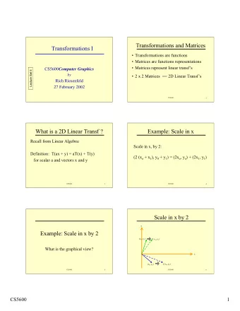
Earlier I promised Solving for a Transformation T 3: Solve for transformation T (e.g. such that p1 ≡ T p2 ) that fits the matches well

Before Anything Else, Remember You, with your The computer gigantic brain, see: sees: You should expect noise (not at quite the right pixel) and outliers (random matches)

Today • How do we fit models (i.e., a parameteric representation of data that’s smaller than the data) to data? • How do we handle: • Noise – least squares / total least squares • Outliers – RANSAC (random sample consensus) • Multiple models – Hough Transform (can also make RANSAC handle this with some effort)

Working Example: Lines • We’ll handle lines as our models today since you should be familiar with them • Next class will cover more complex models. I promise we’ll eventually stitch images together • You can apply today’s techniques on next class’s models

Model Fitting Need three ingredients Data: what data are we trying to explain with a model? Model: what’s the compressed, parametric form of the data? Objective function: given a prediction, how do we evaluate how correct it is?

Example: Least-Squares Fitting a line to data Data: (x 1 ,y 1 ), (x 2 ,y 2 ), …, ( x k ,y k ) Model: (m,b) y i =mx i +b Or ( w ) y i = w T x i Objective function: (y i - w T x i ) 2

Least-Squares Setup 𝑙 2 𝑧 𝑗 − 𝒙 𝑈 𝒚 𝒋 2 𝒁 − 𝒀𝒙 2 ෍ 𝑗=1 𝑧 1 𝑦 1 1 𝑛 ⋮ ⋮ 1 𝒁 = 𝒀 = 𝒙 = 𝑐 𝑧 𝑙 𝑦 𝑙 1 Note: I’m writing the most general form here since we’ll do it in general and you can make it specific if you’d like.

Solving Least-Squares 2 𝒁 − 𝒀𝒙 2 𝜖 2 = 2𝒀 𝑼 𝒀𝒙 − 2𝒀 𝑼 𝒁 𝜖𝒙 𝒁 − 𝒀𝒙 2 𝟏 = 2𝒀 𝑼 𝒀𝒙 − 2𝒀 𝑼 𝒁 Recall: derivative is 0 at a maximum / 𝒀 𝑼 𝒀𝒙 = 𝒀 𝑼 𝒁 minimum. Same is true about gradients. −𝟐 𝒀 𝑼 𝒁 𝒙 = 𝒀 𝑼 𝒀 Aside: 0 is a vector of 0s. 1 is a vector of 1s.

Derivation for the Curious = 𝒁 − 𝒀𝒙 𝑈 𝒁 − 𝒀𝒙 2 𝒁 − 𝒀𝒙 2 = 𝒁 𝑼 𝒁 − 𝟑𝒙 𝑼 𝒀 𝑼 𝒁 + 𝒀𝒙 𝑼 𝒀𝒙 𝜖 𝜖𝒙 𝒀𝒙 𝑈 𝐘𝐱 = 𝟑𝐘 𝐔 𝐘𝐱 𝜖 𝒀𝒙 𝑼 𝒀𝒙 = 2 𝜖𝒙 𝜖 2 = 0 − 2𝒀 𝑼 𝒁 + 2𝒀 𝑼 𝒀𝒙 𝒁 − 𝒀𝒙 2 𝜖𝒙 = 2𝒀 𝑼 𝒀𝒙 − 2𝒀 𝑼 𝒁

Two Solutions to Getting W In One Go Iteratively Implicit form Recall: gradient is also (normal equations) direction that makes function go up the most. 𝒀 𝑼 𝒀𝒙 = 𝒀 𝑼 𝒁 What could we do? Explicit form 𝒙 𝟏 = 𝟏 (don’t do this) 𝜖 2 −𝟐 𝒀 𝑼 𝒁 𝒙 𝒋+𝟐 = 𝒙 𝒋 − 𝜹 𝜖𝒙 𝒁 − 𝒀𝒙 2 𝒙 = 𝒀 𝑼 𝒀

What’s The Problem? • Vertical lines impossible! • Not rotationally invariant: the line will change depending on orientation of points

Alternate Formulation Recall: 𝑏𝑦 + 𝑐𝑧 + 𝑑 = 0 𝒎 𝑈 𝒒 = 0 𝒎 ≡ [𝑏, 𝑐, 𝑑] 𝒒 ≡ [𝑦, 𝑧, 1] Can always rescale l. Pick a,b,d such that 2 = 2 = 1 𝒐 2 𝑏, 𝑐 2 𝑒 = −𝑑

Alternate Formulation Now: 𝑏𝑦 + 𝑐𝑧 − 𝑒 = 0 𝒐 𝑼 𝑦, 𝑧 − 𝑒 = 0 Point to line distance: 𝒐 𝑈 𝑦, 𝑧 − 𝑒 𝒐 = 𝑏, 𝑐 = 𝒐 𝑼 𝑦, 𝑧 − 𝑒 2 = 1 𝑏, 𝑐 2 2 𝒐 2

Total Least-Squares Fitting a line to data Data: (x 1 ,y 1 ), (x 2 ,y 2 ), …, ( x k ,y k ) Model: ( n ,d), ||n|| 2 = 1 n T [x i ,y i ]-d=0 𝒐 = 𝑏, 𝑐 2 = 1 Objective function: 𝑏, 𝑐 2 ( n T [x i ,y i ]-d) 2

Total Least Squares Setup Figure out objective first, then figure out ||n||=1 𝑙 2 𝒐 𝑼 𝑦, 𝑧 − 𝑒 2 𝒀𝒐 − 𝟐𝑒 2 ෍ 𝑗=1 𝑦 1 𝑧 1 1 𝑏 𝝂 = 1 𝒐 = ⋮ ⋮ 𝑙 𝟐 𝑈 𝒀 𝟐 = 𝒀 = ⋮ 𝑐 𝑦 𝑙 𝑧 𝑙 1 The mean / center of mass of the points: we’ll use it later

Solving Total Least-Squares 2 = 𝒀𝒐 − 𝟐𝑒 𝑈 (𝒀𝒐 − 𝟐𝑒) 𝒀𝒐 − 𝟐𝑒 2 = 𝒀𝒐 𝑼 𝒀𝒐 − 2𝑒𝟐 𝑼 𝒀𝒐 + 𝑒 𝟑 𝟐 𝑼 𝟐 First solve for d at optimum (set to 0) 𝜖 2 = 0 − 2𝟐 𝑼 𝒀𝒐 + 2𝑒𝑙 𝜖𝑒 𝒀𝒐 − 𝟐𝑒 2 0 = −2𝟐 𝑼 𝒀𝒐 + 2𝑒𝑙 0 = −𝟐 𝑼 𝒀𝒐 + 𝑒𝑙 𝑒 = 1 𝑙 𝟐 𝑼 𝒀𝒐 = 𝝂𝒐

Solving Total Least-Squares 2 2 𝑒 = 𝝂𝒐 𝒀𝒐 − 𝟐𝑒 2 = 𝒀𝒐 − 𝟐𝝂𝒐 2 2 = 𝒀 − 𝟐𝝂 𝒐 2 Objective is then: 2 arg min 𝒀 − 𝟐𝝂 𝒐 2 𝒐 =1

Homogeneous Least Squares 2 Eigenvector corresponding to arg min 𝑩𝒘 2 smallest eigenvalue of A T A 2 =1 𝒘 2 Why do we need ||v|| 2 = 1 or some other constraint? Applying it in our case: 𝒐 = smallest_eigenvec( 𝒀 − 𝟐𝝂 𝑼 (𝒀 − 𝟐𝝂)) Note: technically homogeneous only refers to ||Av||=0 but it’s common shorthand in computer vision to refer to the specific problem of ||v||=1

Details For ML-People Matrix we take the eigenvector of looks like: 𝑦 𝑗 − 𝜈 𝑦 2 ෍ ෍ 𝑦 𝑗 − 𝜈 𝑦 𝑧 𝑗 − 𝜈 𝑧 𝑗 𝑗 𝒀 − 𝟐𝝂 𝑼 (𝒀 − 𝟐𝝂) = 2 𝑦 𝑗 − 𝜈 𝑦 𝑧 𝑗 − 𝜈 𝑧 𝑧 𝑗 − 𝜈 𝑧 ෍ ෍ 𝑗 𝑗 This is a scatter matrix or scalar multiple of the covariance matrix. We’re doing PCA, but taking the least principal component to get the normal. Note: If you don’t know PCA, just ignore this slide; it’s to help build connections to people with a background in data science/ML.

Running Least-Squares

Running Least-Squares

Ruining Least Squares

Ruining Least Squares

Ruining Least Squares Way to think of it #1: 2 𝒁 − 𝒀𝑿 2 100^2 >> 10^2: least-squares prefers having no large errors, even if the model is useless overall Way to think of it #2: −1 𝒀 𝑈 𝒁 𝑿 = 𝒀 𝑼 𝒀 Weights are a linear transformation of the output variable: can manipulate W by manipulating Y.

Common Fixes Replace Least-Squares objective Let 𝑭 = 𝒁 − 𝒀𝑿 2 LS/L2/MSE: 𝑭 𝑗 L1: |𝑭 𝑗 | Huber: 1 2 2 𝑭 𝑗 |𝑭 𝑗 | ≤ 𝜀: 𝜀 |𝑭 𝑗 | − 𝜀 |𝑭 𝑗 | > 𝜀: 2

Issues with Common Fixes • Usually complicated to optimize: • Often no closed form solution • Typically not something you could write yourself • Sometimes not convex (no global optimum) • Not simple to extend more complex objectives to things like total-least squares • Typically don’t handle a ton of outliers (e.g., 80% outliers)

Outliers in Computer Vision Single outlier: Many outliers: rare common

Ruining Least Squares Continued

Ruining Least Squares Continued

A Simple, Yet Clever Idea • What we really want : model explains many points “well” • Least Squares : model makes as few big mistakes as possible over the entire dataset • New objective : find model for which error is “small” for as many data points as possible • Method : RANSAC ( RA ndom SA mple C onsensus) M. A. Fischler, R. C. Bolles. Random Sample Consensus: A Paradigm for Model Fitting with Applications to Image Analysis and Automated Cartography. Comm. of the ACM, Vol 24, pp 381-395, 1981.

RANSAC For Lines bestLine, bestCount = None, -1 for trial in range(numTrials): subset = pickPairOfPoints(data) line = totalLeastSquares(subset) E = linePointDistance(data,line) inliers = E < threshold if #inliers > bestCount: bestLine, bestCount = line, #inliers

Running RANSAC Best Lots of outliers! Model: Trial None #1 Best Count: -1

Running RANSAC Best Fit line to 2 Model: random points Trial None #1 Best Count: -1

Running RANSAC Best Point/line distance Model: |n T [x,y] – d| Trial None #1 Best Count: -1

Running RANSAC Best Distance < threshold Model: 14 points satisfy this Trial None #1 Best Count: -1

Running RANSAC Best Distance < threshold Model: 14 points Trial #1 Best Count: 14

Running RANSAC Best Distance < threshold Model: 22 points Trial #2 Best Count: 14

Running RANSAC Best Distance < threshold Model: 22 points Trial #2 Best Count: 22

Running RANSAC Best Distance < threshold Model: 10 Trial #3 Best Count: 22

Running RANSAC Best Model: … Trial #3 Best Count: 22

Running RANSAC Best Distance < threshold Model: 76 Trial #9 Best Count: 22

Running RANSAC Best Distance < threshold Model: 76 Trial #9 Best Count: 76

Running RANSAC Best Model: … Trial #9 Best Count: 76

Running RANSAC Best Distance < threshold Model: 22 Trial #100 Best Count: 85

Running RANSAC Final Output of RANSAC: Best Model