Functions and Data Fitting COMPSCI 371D Machine Learning COMPSCI - PowerPoint PPT Presentation
Functions and Data Fitting COMPSCI 371D Machine Learning COMPSCI 371D Machine Learning Functions and Data Fitting 1 / 17 Outline 1 Functions 2 Features 3 Polynomial Fitting: Univariate Least Squares Fitting Choosing a Degree 4
Functions and Data Fitting COMPSCI 371D — Machine Learning COMPSCI 371D — Machine Learning Functions and Data Fitting 1 / 17
Outline 1 Functions 2 Features 3 Polynomial Fitting: Univariate Least Squares Fitting Choosing a Degree 4 Polynomial Fitting: Multivariate 5 Limitations of Polynomials 6 The Curse of Dimensionality COMPSCI 371D — Machine Learning Functions and Data Fitting 2 / 17
Functions Functions Everywhere • SPAM A = { all possible emails } Y = { true , false } f : A → Y and y = f ( a ) ∈ Y for a ∈ A • Virtual Tennis A = { all possible video frames } ⊆ R d Y = { body configurations } ⊆ R e • Medical diagnosis, speech recognition, movie recommendation • Predictor = Regressor or Classifier COMPSCI 371D — Machine Learning Functions and Data Fitting 3 / 17
Functions Classic and ML • Classic: • Design features by hand • Design f by hand • ML: Define A , Y Collect T a = { ( a 1 , y 1 ) , . . . , ( a N , y N ) } ⊂ A × Y Choose F Design λ : { all possible T a } → F Train : f = λ ( T a ) Hopefully, y ≈ f ( a ) now and forever • Technical: A can be anything. Too difficult to work with. COMPSCI 371D — Machine Learning Functions and Data Fitting 4 / 17
Features Features • From A to X ∈ R d x = φ ( a ) y = h ( x ) = h ( φ ( a )) = f ( a ) h : X ⊆ R d → Y ⊆ R e H ⊆ { X → Y } T = { ( x 1 , y 1 ) , . . . , ( x N , y N ) } ⊂ X × Y • Just numbers! COMPSCI 371D — Machine Learning Functions and Data Fitting 5 / 17
Features Features for SPAM d = 20 , 000 φ also useful in order to make d smaller or more informative COMPSCI 371D — Machine Learning Functions and Data Fitting 6 / 17
Features Fitting and Learning • Loss ℓ ( y , h ( x )) : Y × Y → R + • Empirical Risk (ER): average loss on T • Fitting and Learning: • Given T ⊂ X × Y with X ⊆ R d H = { h : X → Y } ( hypothesis space ) • Fitting: Choose h ∈ H to minimize ER over T • Learning: Choose h ∈ H to minimize some risk over previously unseen ( x , y ) COMPSCI 371D — Machine Learning Functions and Data Fitting 7 / 17
Features Summary • Features insulate ML from domain vagaries • Loss function insulates ML from price considerations • Empirical Risk (ER) averages loss for h over T • ER measures average performance of h • A learner picks an h ∈ H that minimizes some risk • Data fitting minimizes ER and stops here • ML wants h to do well also tomorrow • The risk for ML is on a bigger set COMPSCI 371D — Machine Learning Functions and Data Fitting 8 / 17
Polynomial Fitting: Univariate Data Fitting: Univariate Polynomials h : R → R h ( x ) = c 0 + c 1 x + . . . + c k x k with c i ∈ R for i = 0 , . . . , k and c k � = 0 • The definition of the structure of h defines the hypothesis space H • T = { ( x 1 , y 1 ) , . . . , ( x N , y N ) } ⊂ R × R • Quadratic loss ℓ ( y , ˆ y ) = ( y − ˆ y ) 2 def � N 1 • ER: L T ( h ) = n = 1 ℓ ( y n , h ( x n )) N • Choosing h is the same as choosing c = [ c 0 , . . . , c k ] T • L T is a quadratic function of c COMPSCI 371D — Machine Learning Functions and Data Fitting 9 / 17
Polynomial Fitting: Univariate Rephrasing the Loss n = 1 [ y n − h ( x n )] 2 = NL T ( h ) = � N � N n = 1 { y n − [ c 0 + c 1 x n + . . . + c k x k n ] } 2 2 � � y 1 − [ c 0 + c 1 x 1 + . . . + c k x k 1 ] � � � . � . = � � . � � � y N − [ c 0 + c 1 x N + . . . + c k x k � N ] � � 2 � � x k y 1 1 x 1 . . . c 0 � � 1 � . . . � . . . − � . . . � � � x k � � y N 1 x N . . . c k � N � = � b − A c � 2 COMPSCI 371D — Machine Learning Functions and Data Fitting 10 / 17
Polynomial Fitting: Univariate Linear System in c c 0 + c 1 x n + . . . + c k x k n = y n A c = b x k 1 x 1 . . . y 1 1 . . . . . . . . A = and b = . . . . x k 1 x N . . . y n N • Where are the unknowns? • Why is this linear? COMPSCI 371D — Machine Learning Functions and Data Fitting 11 / 17
Polynomial Fitting: Univariate Least Squares Fitting Least Squares A c = b ? b ∈ range ( A ) ˆ c � A c − b � 2 c ∈ arg min Thus, we are minimizing the empirical risk L T ( h ) (with the quadratic loss) over the training set COMPSCI 371D — Machine Learning Functions and Data Fitting 12 / 17
Polynomial Fitting: Univariate Choosing a Degree Choosing a Degree 5 5 5 0 0 0 0 1 0 1 0 1 k = 1 k = 3 k = 9 • Underfitting, overfitting, interpolation COMPSCI 371D — Machine Learning Functions and Data Fitting 13 / 17
Polynomial Fitting: Multivariate Data Fitting: Multivariate Polynomials • The story is not very different: h ( x ) = c 0 + c 1 x 1 + c 2 x 2 + c 3 x 2 1 + c 4 x 1 x 2 + c 5 x 2 2 • Polynomial of degree 2 x 2 x 2 1 x 11 x 12 x 11 x 12 y 1 11 12 . . . . . . . . . . . . . . A = and b = . . . . . . . x 2 x 2 1 x N 1 x N 2 x N 1 x N 2 y N N 1 N 2 • The rest is the same • Why are we not done? COMPSCI 371D — Machine Learning Functions and Data Fitting 14 / 17
Limitations of Polynomials Counting Monomials • Monomial of degree k ′ ≤ k : x k 1 1 . . . x k d k 1 + . . . + k d = k ′ where d • How many are there? � d + k ′ � m ( d , k ′ ) = k ′ (See an Appendix for a proof) COMPSCI 371D — Machine Learning Functions and Data Fitting 15 / 17
Limitations of Polynomials Asymptotics: Too Many Monomials � d + k = ( d + k )! = ( d + k ) ( d + k − 1 ) ... ( d + 1 ) � m ( d , k ) = k d ! k ! k ! k fixed: O ( d k ) d fixed: O ( k d ) • When k is O ( d ) , look at m ( d , d ) : √ O ( 4 d / m ( d , d ) is d ) • Except when k = 1 or d = 1, growth is polynomial (with typically large power) or exponential (if k and d grow together) COMPSCI 371D — Machine Learning Functions and Data Fitting 16 / 17
The Curse of Dimensionality The Curse of Dimensionality • A large d is trouble regardless of H • We want T to be “representative” • “Filling” R d with N samples X = [ 0 , 1 ] 2 ⊂ R 2 10 bins per dimension, 10 2 bins total X = [ 0 , 1 ] d ⊂ R d 10 bins per dimension, 10 d bins total • d is often hundreds or thousands (SPAM d ≈ 20 , 000) • 10 80 atoms in the universe • We will always have too few data points COMPSCI 371D — Machine Learning Functions and Data Fitting 17 / 17
Recommend
More recommend
Explore More Topics
Stay informed with curated content and fresh updates.
