Unit 1: Data Fitting Motivation Data fitting: Construct a - PowerPoint PPT Presentation
Unit 1: Data Fitting Motivation Data fitting: Construct a continuous function that represents discrete data, fundamental topic in Scientific Computing We will study two types of data fitting interpolation: Fit the data points exactly
Polynomial Interpolation Error Now, let e ( x ) ≡ f ( x ) − q ( x ) ◮ e has 3 roots in [ x 0 , x 1 ], i.e. at x = x 0 , ˆ x , x 1 ◮ Therefore e ′ has 2 roots in ( x 0 , x 1 ) (by Rolle’s theorem) ◮ Therefore e ′′ has 1 root in ( x 0 , x 1 ) (by Rolle’s theorem) Let θ ∈ ( x 0 , x 1 ) be such that 4 e ′′ ( θ ) = 0 Then e ′′ ( θ ) = f ′′ ( θ ) − q ′′ ( θ ) 0 = 1 ( θ ) − λ d 2 f ′′ ( θ ) − p ′′ = d θ 2 ( θ − x 0 )( θ − x 1 ) f ′′ ( θ ) − 2 λ = hence λ = 1 2 f ′′ ( θ ) 4 Note that θ is a function of ˆ x
Polynomial Interpolation Error Hence, we get x − x 1 ) = 1 2 f ′′ ( θ )(ˆ f (ˆ x ) − p 1 (ˆ x ) = λ (ˆ x − x 0 )(ˆ x − x 0 )(ˆ x − x 1 ) for any ˆ x ∈ ( x 0 , x 1 ) (recall that ˆ x was chosen arbitrarily) This argument can be generalized to n > 1 to give f ( x ) − p n ( x ) = f ( n +1) ( θ ) ( n +1)! ( x − x 0 ) . . . ( x − x n ) for some θ ∈ ( a , b )
Polynomial Interpolation Error For any x ∈ [ a , b ], this theorem gives us the error bound M n +1 | f ( x ) − p n ( x ) | ≤ ( n + 1)! max x ∈ [ a , b ] | ( x − x 0 ) . . . ( x − x n ) | , where M n +1 = max θ ∈ [ a , b ] | f n +1 ( θ ) | If 1 / ( n + 1)! → 0 faster than M n +1 max x ∈ [ a , b ] | ( x − x 0 ) . . . ( x − x n ) | → ∞ then p n → f Unfortunately, this is not always the case!
Runge’s Phenomenon A famous pathological example of the difficulty of interpolation at equally spaced points is Runge’s Phenomenon Consider f ( x ) = 1 / (1 + 25 x 2 ) for x ∈ [ − 1 , 1] 1 1 0.8 0.8 0.6 0.6 0.4 0.2 0.4 0 0.2 −0.2 −0.4 0 −0.6 −0.2 −0.8 −0.4 −1 −1 −0.8 −0.6 −0.4 −0.2 0 0.2 0.4 0.6 0.8 1 −1 −0.8 −0.6 −0.4 −0.2 0 0.2 0.4 0.6 0.8 1 1 2 0.5 0 0 −2 −0.5 −4 −1 −1.5 −6 −2 −8 −2.5 −10 −3 −12 −3.5 −4 −14 −1 −0.8 −0.6 −0.4 −0.2 0 0.2 0.4 0.6 0.8 1 −1 −0.8 −0.6 −0.4 −0.2 0 0.2 0.4 0.6 0.8 1
Runge’s Phenomenon Note that of course p n fits the evenly spaced samples exactly But we are now also interested in the maximum error between f and its polynomial interpolant p n That is, we want max x ∈ [ − 1 , 1] | f ( x ) − p n ( x ) | to be small! This is generally referred to as the “infinity norm” or the “max norm”: � f − p n � ∞ ≡ x ∈ [ − 1 , 1] | f ( x ) − p n ( x ) | max
Runge’s Phenomenon Interpolating Runge’s function at evenly spaced points leads to exponential growth of infinity norm error! We would like to construct an interpolant of f such that this kind of pathological behavior is impossible
Minimizing Interpolation Error To do this, we recall our error equation f ( x ) − p n ( x ) = f n +1 ( θ ) ( n + 1)!( x − x 0 ) . . . ( x − x n ) We focus our attention on the polynomial ( x − x 0 ) . . . ( x − x n ), since we can choose the interpolation points Intuitively, we should choose x 0 , x 1 , . . . , x n such that � ( x − x 0 ) . . . ( x − x n ) � ∞ is as small as possible
Interpolation at Chebyshev Points Result from Approximation Theory: For x ∈ [ − 1 , 1], the minimum value of � ( x − x 0 ) . . . ( x − x n ) � ∞ is 1 / 2 n , achieved by the polynomial T n +1 ( x ) / 2 n T n +1 ( x ) is the Chebyshev poly. (of the first kind) of order n + 1 ( T n +1 has leading coefficient of 2 n , hence T n +1 ( x ) / 2 n is monic) Chebyshev polys “equi-oscillate” between − 1 and 1, hence it’s not surprising that they are related to the minimum infinity norm 1.5 1 0.5 0 −0.5 −1 −1.5 −1 −0.5 0 0.5 1
Interpolation at Chebyshev Points Chebyshev polynomials are defined for x ∈ [ − 1 , 1] by T n ( x ) = cos( n cos − 1 x ) , n = 0 , 1 , 2 , . . . Or equivalently 5 , the recurrence relation, T 0 ( x ) = 1, T 1 ( x ) = x , T n +1 ( x ) = 2 xT n ( x ) − T n − 1 ( x ), n = 1 , 2 , 3 , . . . To set ( x − x 0 ) . . . ( x − x n ) = T n +1 ( x ) / 2 n , we choose interpolation points to be the roots of T n +1 Exercise: Show that the roots of T n are given by x j = cos((2 j − 1) π/ 2 n ), j = 1 , . . . , n 5 Equivalence can be shown using trig. identities for T n +1 and T n − 1
Interpolation at Chebyshev Points We can combine these results to derive an error bound for interpolation at “Chebyshev points” Generally speaking, with Chebyshev interpolation, p n converges to any smooth f very rapidly! e.g. Runge function: Interpolation at 32 Chebyshev points 1 0.9 0.8 0.7 0.6 0.5 0.4 0.3 0.2 0.1 0 −1 −0.8 −0.6 −0.4 −0.2 0 0.2 0.4 0.6 0.8 1 If we want to interpolate on an arbitrary interval, we can map Chebyshev points from [ − 1 , 1] to [ a , b ]
Interpolation at Chebyshev Points Note that convergence rates depend on smoothness of f —precise statements about this can be made, outside the scope of AM205 ⇒ faster convergence 6 In general, smoother f = e.g. [ ch inter.py ] compare convergence of Chebyshev interpolation of Runge’s function (smooth) and f ( x ) = | x | (not smooth) 0 10 Runge abs. val. −1 10 −2 10 −3 10 −4 10 −5 10 0 10 20 30 40 50 60 n 6 For example, if f is analytic, we get exponential convergence!
Another View on Interpolation Accuracy We have seen that the interpolation points we choose have an enormous effect on how well our interpolant approximates f The choice of Chebyshev interpolation points was motivated by our interpolation error formula for f ( x ) − p n ( x ) But this formula depends on f — we would prefer to have a measure of interpolation accuracy that is independent of f This would provide a more general way to compare the quality of interpolation points . . . This is provided by the Lebesgue constant
Lebesgue Constant Let X denote a set of interpolation points, X ≡ { x 0 , x 1 , . . . , x n } ⊂ [ a , b ] A fundamental property of X is its Lebesgue constant, Λ n ( X ), n � Λ n ( X ) = max | L k ( x ) | x ∈ [ a , b ] k =0 The L k ∈ P n are the Lagrange polynomials associated with X , hence Λ n is also a function of X Λ n ( X ) ≥ 1, why?
Lebesgue Constant Think of polynomial interpolation as a map, I n , where I n : C [ a , b ] → P n [ a , b ] I n ( f ) is the degree n polynomial interpolant of f ∈ C [ a , b ] at the interpolation points X Exercise: Convince yourself that I n is linear ( e.g. use the Lagrange interpolation formula) The reason that the Lebesgue constant is interesting is because it bounds the “operator norm” of I n : �I n ( f ) � ∞ sup ≤ Λ n ( X ) � f � ∞ f ∈ C [ a , b ]
Lebesgue Constant Proof: � � n n � � � � �I n ( f ) � ∞ = � f ( x k ) L k � ∞ = max f ( x k ) L k ( x ) � � � � x ∈ [ a , b ] k =0 � k =0 � n � ≤ max | f ( x k ) || L k ( x ) | x ∈ [ a , b ] k =0 n � � � ≤ k =0 , 1 ,..., n | f ( x k ) | max max | L k ( x ) | x ∈ [ a , b ] k =0 n � ≤ � f � ∞ max | L k ( x ) | x ∈ [ a , b ] k =0 = � f � ∞ Λ n ( X ) Hence �I n ( f ) � ∞ �I n ( f ) � ∞ ≤ Λ n ( X ) , so sup ≤ Λ n ( X ) . � f � ∞ � f � ∞ f ∈ C [ a , b ]
Lebesgue Constant The Lebesgue constant allows us to bound interpolation error in terms of the smallest possible error from P n Let p ∗ n ∈ P n denote the best infinity-norm approximation to f , i.e. � f − p ∗ n � ∞ ≤ � f − w � ∞ for all w ∈ P n Some facts about p ∗ n : ◮ � p ∗ n − f � ∞ → 0 as n → ∞ for any continuous f ! (Weierstraß approximation theorem) ◮ p ∗ n ∈ P n is unique ◮ In general, p ∗ n is unknown
Bernstein interpolation The Bernstein polynomials on [0 , 1] are � n � x m (1 − x ) n − m . b m , n ( x ) = m For a function f on the [0 , 1], the approximating polynomial is n � m � � B n ( f )( x ) = f b m , n ( x ) . n m =0 Bernstein interpolation is impractical for normal use, and converges extremely slowly. However, it has robust convergence properties, which can be used to prove the Weierstraß approximation theorem. See a textbook on real analysis for a full discussion. 7 7 e.g. Elementary Analysis by Kenneth A. Ross
Bernstein interpolation Bernstein polynomials 1 f ( x ) 0.5 0 -0.5 -1 0 0.2 0.4 0.6 0.8 1 x
Bernstein interpolation 0.7 0.6 0.5 0.4 0.3 0.2 0.1 0 -0.1 Bernstein polynomials g ( x ) -0.2 0 0.2 0.4 0.6 0.8 1 x
Lebesgue Constant Then, we can relate interpolation error to � f − p ∗ n � ∞ as follows: � f − p ∗ n � ∞ + � p ∗ � f − I n ( f ) � ∞ ≤ n − I n ( f ) � ∞ � f − p ∗ n � ∞ + �I n ( p ∗ = n ) − I n ( f ) � ∞ � f − p ∗ n � ∞ + �I n ( p ∗ = n − f ) � ∞ n � ∞ + �I n ( p ∗ n − f ) � ∞ � f − p ∗ � f − p ∗ = n � ∞ � p ∗ n − f � ∞ � f − p ∗ n � ∞ + Λ n ( X ) � f − p ∗ ≤ n � ∞ (1 + Λ n ( X )) � f − p ∗ = n � ∞
Lebesgue Constant Small Lebesgue constant means that our interpolation can’t be much worse that the best possible polynomial approximation! [ lsum.py ] Now let’s compare Lebesgue constants for equispaced ( X equi ) and Chebyshev points ( X cheb )
Lebesgue Constant Plot of � 10 k =0 | L k ( x ) | for X equi and X cheb (11 pts in [ − 1 , 1]) 30 2.5 25 20 2 15 10 1.5 5 0 1 −1 −0.5 0 0.5 1 −1 −0.5 0 0.5 1 Λ 10 ( X equi ) ≈ 29 . 9 Λ 10 ( X cheb ) ≈ 2 . 49
Lebesgue Constant Plot of � 20 k =0 | L k ( x ) | for X equi and X cheb (21 pts in [ − 1 , 1]) 12000 3 2.8 10000 2.6 2.4 8000 2.2 6000 2 1.8 4000 1.6 1.4 2000 1.2 0 1 −1 −0.5 0 0.5 1 −1 −0.5 0 0.5 1 Λ 20 ( X equi ) ≈ 10 , 987 Λ 20 ( X cheb ) ≈ 2 . 9
Lebesgue Constant Plot of � 30 k =0 | L k ( x ) | for X equi and X cheb (31 pts in [ − 1 , 1]) 6 7 x 10 3.5 6 3 5 2.5 4 3 2 2 1.5 1 0 1 −1 −0.5 0 0.5 1 −1 −0.5 0 0.5 1 Λ 30 ( X equi ) ≈ 6 , 600 , 000 Λ 30 ( X cheb ) ≈ 3 . 15
Lebesgue Constant The explosive growth of Λ n ( X equi ) is an explanation for Runge’s phenomenon 8 It has been shown that as n → ∞ , 2 n Λ n ( X equi ) ∼ BAD! en log n whereas Λ n ( X cheb ) < 2 π log( n + 1) + 1 GOOD! Important open mathematical problem: What is the optimal set of interpolation points ( i.e. what X minimizes Λ n ( X ))? 8 Runge’s function f ( x ) = 1 / (1 + 25 x 2 ) excites the “worst case” behavior allowed by Λ n ( X equi )
Summary It is helpful to compare and contrast the two key topics we’ve considered so far in this chapter 1. Polynomial interpolation for fitting discrete data: ◮ We get “zero error” regardless of the interpolation points, i.e. we’re guaranteed to fit the discrete data ◮ Should use Lagrange polynomial basis (diagonal system, well-conditioned) 2. Polynomial interpolation for approximating continuous functions: ◮ For a given set of interpolating points, uses the methodology from 1 above to construct the interpolant ◮ But now interpolation points play a crucial role in determining the magnitude of the error � f − I n ( f ) � ∞
Piecewise Polynomial Interpolation We can’t always choose our interpolation points to be Chebyshev, so another way to avoid “blow up” is via piecewise polynomials Idea is simple: Break domain into subdomains, apply polynomial interpolation on each subdomain (interp. pts. now called “knots”) Recall piecewise linear interpolation, also called “linear spline” 1 0.9 0.8 0.7 0.6 0.5 0.4 0.3 0.2 0.1 0 −1 −0.5 0 0.5 1
Piecewise Polynomial Interpolation With piecewise polynomials, we avoid high-order polynomials hence we avoid “blow-up” However, we clearly lose smoothness of the interpolant Also, can’t do better than algebraic convergence 9 9 Recall that for smooth functions Chebyshev interpolation gives exponential convergence with n
Splines Splines are a popular type of piecewise polynomial interpolant In general, a spline of degree k is a piecewise polynomial that is continuously differentiable k − 1 times Splines solve the “loss of smoothness” issue to some extent since they have continuous derivatives Splines are the basis of CAD software (AutoCAD, SolidWorks), also used in vector graphics, fonts, etc. 10 (The name “spline” comes from a tool used by ship designers to draw smooth curves by hand) 10 CAD software uses NURB splines, font definitions use B´ ezier splines
Splines We focus on a popular type of spline: Cubic spline ∈ C 2 [ a , b ] Continuous second derivatives = ⇒ looks smooth to the eye Example: Cubic spline interpolation of Runge function 1 0.9 0.8 0.7 0.6 0.5 0.4 0.3 0.2 0.1 0 −1 −0.5 0 0.5 1
Cubic Splines: Formulation Suppose we have knots x 0 , . . . , x n , then cubic on each interval [ x i − 1 , x i ] = ⇒ 4 n parameters in total Let s denote our cubic spline, and suppose we want to interpolate the data { f i , i = 0 , 1 , . . . , n } We must interpolate at n + 1 points, s ( x i ) = f i , which provides two equations per interval = ⇒ 2 n equations for interpolation Also, s ′ − ( x i ) = s ′ + ( x i ), i = 1 , . . . , n − 1 = ⇒ n − 1 equations for continuous first derivative And, s ′′ − ( x i ) = s ′′ + ( x i ), i = 1 , . . . , n − 1 = ⇒ n − 1 equations for continuous second derivative Hence 4 n − 2 equations in total
Cubic Splines We are short by two conditions! There are many ways to make up the last two, e.g. ◮ Natural cubic spline: Set s ′′ ( x 0 ) = s ′′ ( x n ) = 0 ◮ “Not-a-knot spline” 11 : Set s ′′′ − ( x 1 ) = s ′′′ + ( x 1 ) and s ′′′ − ( x n − 1 ) = s ′′′ + ( x n − 1 ) ◮ Or we can choose any other two equations we like ( e.g. set two of the spline parameters to zero) 12 See examples: [ spline.py ] & [ spline2.py ] 11 “Not-a-knot” because all derivatives of s are continuous at x 1 and x n − 1 12 As long as they are linearly independent from the first 4 n − 2 equations
Linear Least Squares: The Problem Formulation Recall that it can be advantageous to not fit data points exactly ( e.g. due to experimental error), we don’t want to “overfit” Suppose we want to fit a cubic polynomial to 11 data points 4.2 4 3.8 3.6 y 3.4 3.2 3 2.8 0 0.5 1 1.5 2 x Question: How do we do this?
The Problem Formulation Suppose we have m constraints and n parameters with m > n ( e.g. m = 11, n = 4 on previous slide) In terms of linear algebra, this is an overdetermined system Ab = y , where A ∈ R m × n , b ∈ R n (parameters), y ∈ R m (data) A y = b i.e. we have a “tall, thin” matrix A
The Problem Formulation In general, cannot be solved exactly (hence we will write Ab ≃ y ); instead our goal is to minimize the residual, r ( b ) ∈ R m r ( b ) ≡ y − Ab A very effective approach for this is the method of least squares: 13 Find parameter vector b ∈ R n that minimizes � r ( b ) � 2 As we shall see, we minimize the 2-norm above since it gives us a differentiable function (we can then use calculus) 13 Developed by Gauss and Legendre for fitting astronomical observations with experimental error
The Normal Equations �� n i =1 r i ( b ) 2 Goal is to minimize � r ( b ) � 2 , recall that � r ( b ) � 2 = Since minimizing b is the same for � r ( b ) � 2 and � r ( b ) � 2 2 , we consider the differentiable “objective function” φ ( b ) = � r ( b ) � 2 2 � r � 2 2 = r T r = ( y − Ab ) T ( y − Ab ) φ ( b ) = y T y − y T Ab − b T A T y + b T A T Ab = y T y − 2 b T A T y + b T A T Ab = where last line follows from y T Ab = ( y T Ab ) T , since y T Ab ∈ R φ is a quadratic function of b , and is non-negative, hence a minimum must exist, (but not nec. unique, e.g. f ( b 1 , b 2 ) = b 2 1 )
The Normal Equations To find minimum of φ ( b ) = y T y − 2 b T A T y + b T A T Ab , differentiate with respect to b and set to zero 14 First, let’s differentiate b T A T y with respect to b That is, we want ∇ ( b T c ) where c ≡ A T y ∈ R n : n ∂ � b T c = ( b T c ) = c i = ⇒ ∇ ( b T c ) = c b i c i = ⇒ ∂ b i i =1 Hence ∇ ( b T A T y ) = A T y 14 We will discuss numerical optimization of functions of many variables in detail in Unit IV
The Normal Equations Next consider ∇ ( b T A T Ab ) (note A T A is symmetric) Consider b T Mb for symmetric matrix M ∈ R n × n � n � b T Mb = b T � m (: , j ) b j j =1 From the product rule n ∂ � ∂ b k ( b T Mb ) e T m (: , j ) b j + b T m (: , k ) = k j =1 n � m ( k , j ) b j + b T m (: , k ) = j =1 m ( k , :) b + b T m (: , k ) = = 2 m ( k , :) b , where the last line follows from symmetry of M Therefore, ∇ ( b T Mb ) = 2 Mb , so that ∇ ( b T A T Ab ) = 2 A T Ab
The Normal Equations Putting it all together, we obtain ∇ φ ( b ) = − 2 A T y + 2 A T Ab We set ∇ φ ( b ) = 0 to obtain − 2 A T y + 2 A T Ab = 0 = ⇒ A T Ab = A T y This square n × n system A T Ab = A T y is known as the normal equations
The Normal Equations For A ∈ R m × n with m > n , A T A is singular if and only if A is rank-deficient. 15 Proof: ( ⇒ ) Suppose A T A is singular. ∃ z � = 0 such that A T Az = 0. Hence z T A T Az = � Az � 2 2 = 0, so that Az = 0. Therefore A is rank-deficient. ( ⇐ ) Suppose A is rank-deficient. ∃ z � = 0 such that Az = 0, hence A T Az = 0, so that A T A is singular. 15 Recall A ∈ R m × n , m > n is rank-deficient if columns are not L.I., i.e. ∃ z � = 0 s.t. Az = 0
The Normal Equations Hence if A has full rank ( i.e. rank( A ) = n ) we can solve the normal equations to find the unique minimizer b However, in general it is a bad idea to solve the normal equations directly, because it is not as numerically stable as some alternative methods Question: If we shouldn’t use normal equations, how do we actually solve least-squares problems ?
Least-squares polynomial fit Find least-squares fit for degree 11 polynomial to 50 samples of y = cos(4 x ) for x ∈ [0 , 1] Let’s express the best-fit polynomial using the monomial basis: p ( x ; b ) = � 11 k =0 b k x k (Why not use the Lagrange basis? Lagrange loses its nice properties here since m > n , so we may as well use monomials) The i th condition we’d like to satisfy is p ( x i ; b ) = cos(4 x i ) = ⇒ over-determined system with “50 × 12 Vandermonde matrix”
Least-squares polynomial fit [ lfit.py ] But solving the normal equations still yields a small residual, hence we obtain a good fit to the data � r ( b normal ) � 2 = � y − Ab normal � 2 = 1 . 09 × 10 − 8 � r ( b lst.sq. ) � 2 = � y − Ab lst.sq. � 2 = 8 . 00 × 10 − 9
Non-polynomial Least-squares fitting So far we have dealt with approximations based on polynomials, but we can also develop non-polynomial approximations We just need the model to depend linearly on parameters Example [ np lfit.py ]: Approximate e − x cos(4 x ) using f n ( x ; b ) ≡ � n k = − n b k e kx (Note that f n is linear in b : f n ( x ; γ a + σ b ) = γ f n ( x ; a ) + σ f n ( x ; b ))
Non-polynomial Least-squares fitting 3 terms in approximation 1.5 e −x cos(4x) 1 samples best fit 0.5 0 −0.5 −1 −1.5 −2 −2.5 −3 −1 −0.5 0 0.5 1 � r ( b ) � 2 = 4 . 16 × 10 − 1 n = 1 , � b � 2
Non-polynomial Least-squares fitting 7 terms in approximation 1.5 e −x cos(4x) samples 1 best fit 0.5 0 −0.5 −1 −1.5 −2 −2.5 −1 −0.5 0 0.5 1 � r ( b ) � 2 = 1 . 44 × 10 − 3 n = 3 , � b � 2
Non-polynomial Least-squares fitting 11 terms in approximation 1.5 e −x cos(4x) samples 1 best fit 0.5 0 −0.5 −1 −1.5 −2 −2.5 −1 −0.5 0 0.5 1 � r ( b ) � 2 = 7 . 46 × 10 − 6 n = 5 , � b � 2
Pseudoinverse Recall that from the normal equations we have: A T Ab = A T y This motivates the idea of the “pseudoinverse” for A ∈ R m × n : A + ≡ ( A T A ) − 1 A T ∈ R n × m Key point: A + generalizes A − 1 , i.e. if A ∈ R n × n is invertible, then A + = A − 1 Proof: A + = ( A T A ) − 1 A T = A − 1 ( A T ) − 1 A T = A − 1
Pseudoinverse Also: ◮ Even when A is not invertible we still have still have A + A = I ◮ In general AA + � = I (hence this is called a “left inverse”) And it follows from our definition that b = A + y , i.e. A + ∈ R n × m gives the least-squares solution Note that we define the pseudoinverse differently in different contexts
Underdetermined Least Squares So far we have focused on overconstrained systems (more constraints than parameters) But least-squares also applies to underconstrained systems: Ab = y with A ∈ R m × n , m < n b y A = i.e. we have a “short, wide” matrix A
Underdetermined Least Squares For φ ( b ) = � r ( b ) � 2 2 = � y − Ab � 2 2 , we can apply the same argument as before ( i.e. set ∇ φ = 0) to again obtain A T Ab = A T y But in this case A T A ∈ R n × n has rank at most m (where m < n ), why? Therefore A T A must be singular! Typical case: There are infinitely vectors b that give r ( b ) = 0, we want to be able to select one of them
Underdetermined Least Squares First idea, pose as a constrained optimization problem to find the feasible b with minimum 2-norm: b T b minimize subject to Ab = y This can be treated using Lagrange multipliers (discussed later in the Optimization section) Idea is that the constraint restricts us to an ( n − m )-dimensional hyperplane of R n on which b T b has a unique minimum
Underdetermined Least Squares We will show later that the Lagrange multiplier approach for the above problem gives: b = A T ( AA T ) − 1 y As a result, in the underdetermined case the pseudoinverse is defined as A + = A T ( AA T ) − 1 ∈ R n × m Note that now AA + = I , but A + A � = I in general ( i.e. this is a “right inverse”)
Underdetermined Least Squares Here we consider an alternative approach for solving the underconstrained case Let’s modify φ so that there is a unique minimum! For example, let φ ( b ) ≡ � r ( b ) � 2 2 + � Sb � 2 2 where S ∈ R n × n is a scaling matrix This is called regularization: we make the problem well-posed (“more regular”) by modifying the objective function
Underdetermined Least Squares Calculating ∇ φ = 0 in the same way as before leads to the system ( A T A + S T S ) b = A T y We need to choose S in some way to ensure ( A T A + S T S ) is invertible Can be proved that if S T S is positive definite then ( A T A + S T S ) is invertible Simplest positive definite regularizer: S = µ I ∈ R n × n for µ ∈ R > 0
Underdetermined Least Squares Example [ under lfit.py ]: Find least-squares fit for degree 11 polynomial to 5 samples of y = cos(4 x ) for x ∈ [0 , 1] ⇒ A ∈ R 5 × 12 12 parameters, 5 constraints = We express the polynomial using the monomial basis (can’t use Lagrange since m � = n ): A is a submatrix of a Vandermonde matrix If we naively use the normal equations we see that cond( A T A ) = 4 . 78 × 10 17 , i.e. “singular to machine precision”! Let’s see what happens when we regularize the problem with some different choices of S
Underdetermined Least Squares Find least-squares fit for degree 11 polynomial to 5 samples of y = cos(4 x ) for x ∈ [0 , 1] Try S = 0 . 001 I ( i.e. µ = 0 . 001) 1.5 � r ( b ) � 2 = 1 . 07 × 10 − 4 1 0.5 � b � 2 = 4 . 40 0 −0.5 −1 cond( A T A + S T S ) = 1 . 54 × 10 7 −1.5 0 0.2 0.4 0.6 0.8 1 Fit is good since regularization term is small but condition number is still large
Underdetermined Least Squares Find least-squares fit for degree 11 polynomial to 5 samples of y = cos(4 x ) for x ∈ [0 , 1] Try S = 0 . 5 I ( i.e. µ = 0 . 5) 0.8 � r ( b ) � 2 = 6 . 60 × 10 − 1 0.6 0.4 0.2 0 � b � 2 = 1 . 15 −0.2 −0.4 −0.6 −0.8 cond( A T A + S T S ) = 62 . 3 −1 0 0.2 0.4 0.6 0.8 1 Regularization term now dominates: small condition number and small � b � 2 , but poor fit to the data!
Underdetermined Least Squares Find least-squares fit for degree 11 polynomial to 5 samples of y = cos(4 x ) for x ∈ [0 , 1] Try S = diag (0 . 1 , 0 . 1 , 0 . 1 , 10 , 10 . . . , 10) 1.5 � r ( b ) � 2 = 4 . 78 × 10 − 1 1 0.5 � b � 2 = 4 . 27 0 −0.5 cond( A T A + S T S ) = 5 . 90 × 10 3 −1 0 0.2 0.4 0.6 0.8 1 We strongly penalize b 3 , b 4 , . . . , b 11 , hence the fit is close to parabolic
Underdetermined Least Squares Find least-squares fit for degree 11 polynomial to 5 samples of y = cos(4 x ) for x ∈ [0 , 1] 1.5 1 � r ( b ) � 2 = 1 . 03 × 10 − 15 0.5 0 −0.5 � b � 2 = 7 . 18 −1 −1.5 0 0.2 0.4 0.6 0.8 1 Python routine gives Lagrange multiplier based solution, hence satisfies the constraints to machine precision
Nonlinear Least Squares So far we have looked at finding a “best fit” solution to a linear system (linear least-squares) A more difficult situation is when we consider least-squares for nonlinear systems Key point: We are referring to linearity in the parameters, not linearity of the model ( e.g. polynomial p n ( x ; b ) = b 0 + b 1 x + . . . + b n x n is nonlinear in x , but linear in b !) In nonlinear least-squares, we fit functions that are nonlinear in the parameters
Nonlinear Least Squares: Example Example: Suppose we have a radio transmitter at ˆ b = (ˆ b 1 , ˆ b 2 ) somewhere in [0 , 1] 2 ( × ) Suppose that we have 10 receivers at locations 2 ) ∈ [0 , 1] 2 ( • ) ( x 1 1 , x 1 2 ) , ( x 2 1 , x 2 2 ) , . . . , ( x 10 1 , x 10 Receiver i returns a measurement for the distance y i to the transmitter, but there is some error/noise ( ǫ ) 1 0.9 x i 0.8 y i + � 0.7 0.6 x 2 0.5 0.4 ˆ b 0.3 0.2 0.1 0 0 0.2 0.4 0.6 0.8 1 x 1
Nonlinear Least Squares: Example Let b be a candidate location for the transmitter The distance from b to ( x i 1 , x i 2 ) is � 1 ) 2 + ( b 2 − x i ( b 1 − x i 2 ) 2 d i ( b ) ≡ We want to choose b to match the data as well as possible, hence minimize the residual r ( b ) ∈ R 10 where r i ( b ) = y i − d i ( b )
Nonlinear Least Squares: Example In this case, r i ( α + β ) � = r i ( α ) + r i ( β ), hence nonlinear least-squares! Define the objective function φ ( b ) = 1 2 � r ( b ) � 2 2 , where r ( b ) ∈ R 10 is the residual vector The 1 / 2 factor in φ ( b ) has no effect on the minimizing b , but leads to slightly cleaner formulae later on
Nonlinear Least Squares As in the linear case, we seek to minimize φ by finding b such that ∇ φ = 0 We have φ ( b ) = 1 � m j =1 [ r j ( b )] 2 2 Hence for the i th component of the gradient vector, we have m m ∂φ = ∂ 1 ∂ r j � r 2 � j = r j ∂ b i ∂ b i 2 ∂ b i j =1 j =1
Nonlinear Least Squares This is equivalent to ∇ φ = J r ( b ) T r ( b ) where J r ( b ) ∈ R m × n is the Jacobian matrix of the residual { J r ( b ) } ij = ∂ r i ( b ) ∂ b j Exercise: Show that J r ( b ) T r ( b ) = 0 reduces to the normal equations when the residual is linear
Nonlinear Least Squares Hence we seek b ∈ R n such that: J r ( b ) T r ( b ) = 0 This has n equations, n unknowns; in general this is a nonlinear system that we have to solve iteratively An important recurring theme is that linear systems can be solved in “one shot,” whereas nonlinear generally requires iteration We will briefly introduce Newton’s method for solving this system and defer detailed discussion until the optimization section
Nonlinear Least Squares Recall Newton’s method for a function of one variable: find x ∈ R such that f ( x ) = 0 Let x k be our current guess, and x k + ∆ x = x , then Taylor expansion gives 0 = f ( x k + ∆ x ) = f ( x k ) + ∆ xf ′ ( x k ) + O ((∆ x ) 2 ) It follows that f ′ ( x k )∆ x ≈ − f ( x k ) (approx. since we neglect the higher order terms) This motivates Newton’s method: f ′ ( x k )∆ x k = − f ( x k ), where x k +1 = x k + ∆ x k
Nonlinear Least Squares This argument generalizes directly to functions of several variables For example, suppose F : R n → R n , then find x s.t. F ( x ) = 0 by J F ( x k )∆ x k = − F ( x k ) where J F is the Jacobian of F , ∆ x k ∈ R n , x k +1 = x k + ∆ x k
Nonlinear Least Squares In the case of nonlinear least squares, to find a stationary point of φ we need to find b such that J r ( b ) T r ( b ) = 0 That is, we want to solve F ( b ) = 0 for F ( b ) ≡ J r ( b ) T r ( b ) We apply Newton’s Method, hence need to find the Jacobian, J F , of the function F : R n → R n
Nonlinear Least Squares Consider ∂ F i ∂ b j (this will be the ij entry of J F ): ∂ F i ∂ � � J r ( b ) T r ( b ) = ∂ b j ∂ b j i m ∂ ∂ r k � = r k ∂ b j ∂ b i k =1 m m ∂ 2 r k ∂ r k ∂ r k � � = + r k ∂ b i ∂ b j ∂ b i ∂ b j k =1 k =1
Gauss–Newton Method It is generally a pain to deal with the second derivatives in the previous formula, second derivatives get messy! Key observation: As we approach a good fit to the data, the residual values r k ( b ), 1 ≤ k ≤ m , should be small ∂ 2 r k Hence we omit the term � m k =1 r k ∂ b i ∂ b j .
Gauss–Newton Method Note that � m ∂ r k ∂ r k ∂ b i = ( J r ( b ) T J r ( b )) ij , so that when the k =1 ∂ b j residual is small J F ( b ) ≈ J r ( b ) T J r ( b ) Then putting all the pieces together, we obtain the iteration: b k +1 = b k + ∆ b k where J r ( b k ) T J r ( b k )∆ b k = − J r ( b k ) T r ( b k ) , k = 1 , 2 , 3 , . . . This is known as the Gauss–Newton Algorithm for nonlinear least squares
Recommend
More recommend
Explore More Topics
Stay informed with curated content and fresh updates.
