Time Series Modelling and Kalman Filters Chris Williams School of - - PowerPoint PPT Presentation

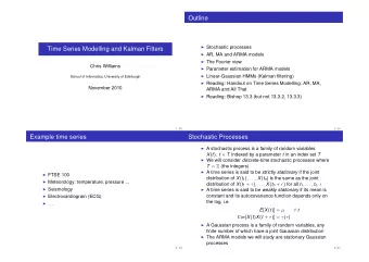
Time Series Modelling and Kalman Filters

Chris Williams

School of Informatics, University of Edinburgh

November 2010

1 / 24

Outline

◮ Stochastic processes ◮ AR, MA and ARMA models ◮ The Fourier view ◮ Parameter estimation for ARMA models ◮ Linear-Gaussian HMMs (Kalman filtering) ◮ Reading: Handout on Time Series Modelling: AR, MA,

ARMA and All That

◮ Reading: Bishop 13.3 (but not 13.3.2, 13.3.3)

2 / 24

Example time series

◮ FTSE 100 ◮ Meteorology: temperature, pressure ... ◮ Seismology ◮ Electrocardiogram (ECG) ◮ . . .

3 / 24

Stochastic Processes

◮ A stochastic process is a family of random variables

X(t), t ∈ T indexed by a parameter t in an index set T

◮ We will consider discrete-time stochastic processes where

T = Z (the integers)

◮ A time series is said to be strictly stationary if the joint

distribution of X(t1), . . . , X(tn) is the same as the joint distribution of X(t1 + τ), . . . , X(tn + τ) for all t1, . . . , tn, τ

◮ A time series is said to be weakly stationary if its mean is

constant and its autocovariance function depends only on the lag, i.e. E[X(t)] = µ ∀ t Cov[X(t)X(t + τ)] = γ(τ)

◮ A Gaussian process is a family of random variables, any

finite number of which have a joint Gaussian distribution

◮ The ARMA models we will study are stationary Gaussian

processes

4 / 24

Autoregressive (AR) Models

◮ Example AR(1)

xt = αxt−1 + wt where wt ∼ N(0, σ2)

◮ By repeated substitution we get

xt = wt + αwt−1 + α2wt−2 + . . .

◮ Hence E[X(t)] = 0, and if |α| < 1 the process is stationary

with Var[X(t)] = (1 + α2 + α4 + . . .)σ2 = σ2 1 − α2

◮ Similarly

Cov[X(t)X(t − k)] = αkVar[X(t − k)] = αkσ2 1 − α2

5 / 24

α = 0.5 α = −0.5

6 / 24

◮ The general case is an AR(p) process

xt =

p

• i=1

αixt−i + wt

◮ Notice how xt is obtainied by a (linear) regression from

xt−1, . . . , xt−p, hence an autoregressive process

◮ Introduce the backward shift operator B, so that

Bxt = xt−1, B2xt = xt−2 etc

◮ Then AR(p) model can be written as

φ(B)xt = wt where φ(B) = (1 − α1B . . . − αpBp)

◮ The condition for stationarity is that all the roots of φ(B) lie

• utside the unit circle

7 / 24

Yule-Walker Equations

xt =

p

• i=1

αixt−i + wt xtxt−k =

p

• i=1

αixt−ixt−k + wtxt−k

◮ Taking expectations (and exploiting stationarity) we obtain

γk =

p

• i=1

αiγk−i k = 1, , 2, . . .

◮ Use p simultaneous equations to obtain the γ’s from the

α’s. For inference, can solve a linear system to obtain the α’s given estimates of the γ’s

◮ Example: AR(1) process, γk = αkγ0

8 / 24

Graphical model illustrating an AR(2) process

. . . . . .

AR2: α1 = 0.2, α2 = 0.1 AR2: α1 = 1.0, α2 = −0.5

9 / 24

Vector AR processes

xt =

p

• i=1

Aixt−i + Gwt where the Ais and G are square matrices

◮ We can in general consider modelling multivariate (as

• pposed to univariate) time series

◮ An AR(2) process can be written as a vector AR(1)

process:

• xt

xt−1

• =

α1 α2 1 xt−1 xt−2

• +

1 wt wt−1

• ◮ In general an AR(p) process can be written as a vector

AR(1) process with a p-dimensional state vector (cf ODEs)

10 / 24

Moving Average (MA) processes

xt =

q

• j=0

βjwt−j (linear filter) = θ(B)wt with scaling so that β0 = 1 and θ(B) = 1 + q

j=1 βjBj

Example: MA(1) process

x’s w’s

11 / 24

◮ We have E[X(t)] = 0, and

Var[X(t)] = (1 + β2

1 + . . . + β2 q)σ2

Cov[X(t)X(t − k)] = E[

q

• j=0

βjwt−j,

q

• i=0

βiwt−k−i] =

• σ2 q−k

j=0 βj+kβj

for k = 0, 1, . . . , q for k > q

◮ Note that covariance “cuts off” for k > q

12 / 24

ARMA(p,q) processes

xt =

p

• i=1

αixt−i +

q

• j=0

βjwt−j φ(B)xt = θ(B)wt

◮ Writing an AR(p) process as a MA(∞) process

φ(B)xt = wt xt = (1 − α1B . . . αpBp)−1wt = (1 + β1B + β2B2 . . .)wt

◮ Similarly a MA(q) process can be written as a AR(∞)

process

◮ Utility of ARMA(p,q) is potential parsimony

13 / 24

The Fourier View

◮ ARMA models are linear time-invariant systems. Hence

sinusoids are their eigenfunctions (Fourier analysis)

◮ This means it is natural to consider the power spectrum of

the ARMA process. The power spectrum S(k) can be determined from the {α}, {β} coefficients

◮ Roughly speaking S(k) is the amount of power allocated

• n average to the eigenfunction e2πikt

◮ This is a useful way to understand some properties of

ARMA processes, but we will not pursue it further here

◮ If you want to know more, see e.g. Chatfield (1989) chapter

7 or Diggle (1990) chapter 4

14 / 24

Parameter Estimation

◮ Let the vector of observations x = (x(t1), . . . , x(tn))T ◮ Estimate and subtract constant offset ˆ

µ if this is non zero

◮ ARMA models driven by Gaussian noise are Gaussian

• processes. Thus the likelihood L(x; α, β) is a multivariate

Gaussian, and we can optimize this wrt the parameters (e.g. by gradient ascent)

◮ AR(p) models,

xt =

p

• i=1

αixt−i + wt can be viewed as the linear regression of xt on the p previous time steps, α and σ2 can be estimated using linear regression

◮ This viewpoint also enables the fitting of nonlinear AR

models

15 / 24

Model Order Selection, References

◮ For a MA(q) process there should be a cut-off in the

autocorrelation function for lags greater than q

◮ For general ARMA models this is model order selection

problem, discussed in an upcoming lecture Some useful books:

◮ The Analysis of Time Series: An Introduction. C. Chatfield,

Chapman and Hall, 4th edition, 1989

◮ Time Series: A Biostatistical Introduction. P

. J. Diggle, Clarendon Press, 1990

16 / 24

Linear-Gaussian HMMs

◮ HMM with continuous state-space and observations ◮ Filtering problem known as Kalman filtering

17 / 24

N

z z z z N A A

1 2 3 3 2 1

. .

C C C C x x x x

◮ Dynamical model

zn+1 = Azn + wn+1 where wn+1 ∼ N(0, Γ) is Gaussian noise, i.e. p(zn+1|zn) ∼ N(Azn, Γ)

18 / 24

◮ Observation model

xn = Czn + vn where vn ∼ N(0, Σ) is Gaussian noise, i.e. p(xn|zn) ∼ N(Czn, Σ)

◮ Initialization

p(z1) ∼ N(µ0, V0)

19 / 24

Inference Problem – filtering

◮ As whole model is Gaussian, only need to compute means and

variances p(zn|x1, . . . , xn) ∼ N(µn, Vn) µn = E[zn|x1, . . . , xn] Vn = E[(zn − µn)(zn − µn)T|x1, . . . , xn]

◮ Recursive update split into two parts ◮ Time update

p(zn|x1, . . . , xn) → p(zn+1|x1, . . . , xn)

◮ Measurement update

p(zn+1|x1, . . . , xn) → p(zn+1|x1, . . . , xn, xn+1)

20 / 24

◮ Time update

zn+1 = Azn + wn+1 thus E[zn+1|x1, . . . xn] = Aµn cov(zn+1|x1, . . . xn)

def

=Pn = AVnAT + Γ

◮ Measurement update (like posterior in Factor Analysis)

µn+1 = Aµn + Kn+1(xn+1 − CAµn) Vn+1 = (I − Kn+1C)Pn where Kn+1 = PnCT(CPnCT + Σ)−1

◮ Kn+1 is known as the Kalman gain matrix

21 / 24

Simple example

zn+1 = zn + wn+1 wn ∼ N(0, 1) xn = zn + vn vn ∼ N(0, 1) p(z1) ∼ N(0, σ2) In the limit σ2 → ∞ we find µ3 = 5x3 + 2x2 + x1 8

◮ Notice how later data has more weight ◮ Compare zn+1 = zn (so that wn has zero variance); then

µ3 = x3 + x2 + x1 3

22 / 24

Applications

Much as a coffee filter serves to keep undesirable grounds out of your morning mug, the Kalman filter is designed to strip unwanted noise out of a stream of

• data. Barry Cipra, SIAM News 26(5) 1993

◮ Navigational and guidance systems ◮ Radar tracking ◮ Sonar ranging ◮ Satellite orbit determination

23 / 24

Extensions

Dealing with non-linearity

◮ The Extended Kalman Filter (EKF)

If xn = f(zn) + vn where f is a non-linear function, can linearize f, e.g. around E[zn|x1, . . . xn−1]. Works for weak non-linearities

◮ For very non-linear problems use sampling methods

(known as particle filters). Example, work of Blake and Isard on tracking, see

http://www.robots.ox.ac.uk/∼vdg/dynamics.html

It is possible to train KFs using a forward-backward algorithm

24 / 24