Overview of Discrete-Time Filters First-order filters Ideal filters - PowerPoint PPT Presentation

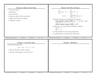
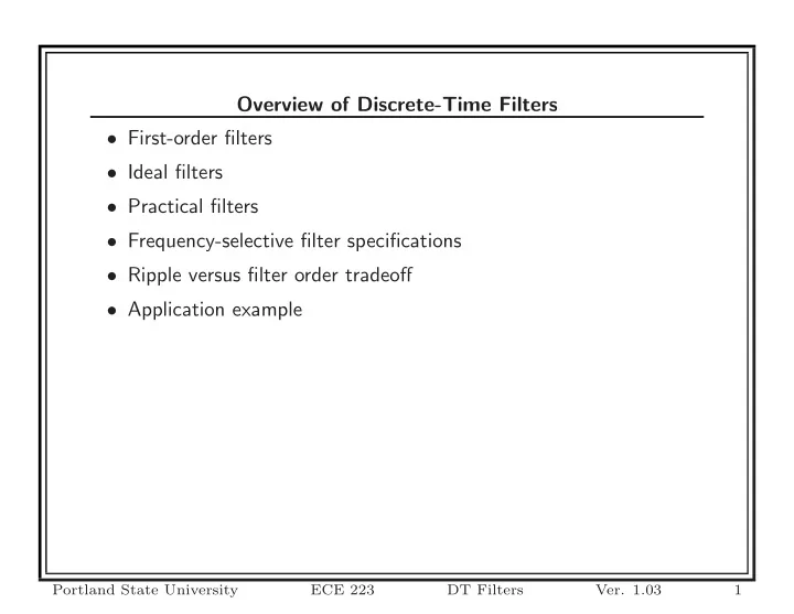
Overview of Discrete-Time Filters • First-order filters • Ideal filters • Practical filters • Frequency-selective filter specifications • Ripple versus filter order tradeoff • Application example Portland State University ECE 223 DT Filters Ver. 1.03 1

Discrete-Time Filters Overview N M � � a k y [ n − k ] = b k x [ n − k ] k =0 k =0 � M k =0 b k e − jwk Y (e jω ) k =0 a k e − jwk X (e jω ) = � N • Discrete-time filters are divided into two categories – Finite impulse response (FIR) : h [ n ] = 0 for some a and b such that −∞ < a < n < b < + ∞ – Infinite impulse response (IIR) : not FIR • Filters that can be described with difference-equations – FIR: N = 0 – IIR: N > 0 • A simple FIR filter is the moving average filter • A simple IIR filter is the first-order lowpass filter Portland State University ECE 223 DT Filters Ver. 1.03 2

Example 1: First-Order Filters Consider the following filter: y [ n ] − ay [ n − 1] = (1 − a ) x [ n ] 1. Solve for the filter’s transfer function 2. Find the cutoff frequency as a function of a Portland State University ECE 223 DT Filters Ver. 1.03 3

Example 1: Workspace Portland State University ECE 223 DT Filters Ver. 1.03 4

Example 1: Ω c versus a 3.5 3 2.5 ω c (rad/sample) 2 1.5 1 0.5 0 0 0.1 0.2 0.3 0.4 0.5 0.6 0.7 0.8 0.9 1 a Portland State University ECE 223 DT Filters Ver. 1.03 5

Example 1: H (e jω ) for various a 1 a=0.1 a=0.2 |H(e j ω )| a=0.3 0.5 a=0.4 a=0.5 a=0.6 0 a=0.7 −3 −2 −1 0 1 2 3 a=0.8 a=0.9 50 ∠ H(e j ω ) ( o ) 0 −50 −3 −2 −1 0 1 2 3 Frequency (rads/sample) Portland State University ECE 223 DT Filters Ver. 1.03 6

Example 1: Filtered Signals Intel Closing Daily Price Over 1 Year 36 34 32 x[n], y 0.1 [n], y 0.6 [n] 30 28 26 24 Raw signal 22 Cutoff:0.56 Cutoff:0.11 20 0 50 100 150 200 Time (day) Portland State University ECE 223 DT Filters Ver. 1.03 7

Example 1: MATLAB Code %function [] = FirstOrderApplied(); close all; d = load(’Intel.txt’); % Closing daily price nd = length(d); x = d(nd:-1:1); % Reorder so first element is oldest data n = (0:nd-1)’; % Discrete time index %============================================================================== % Plot the relationship between cutoff frequency and a %============================================================================== a = 0.00001:0.01:1; wc = acos((1-4*a+a.^2)./(-2*a)); figure FigureSet(1,’LTX’); h = plot(a,wc,’LineWidth’,1.0); ylabel(’\omega_c (rad/sample)’); xlabel(’a’); grid on; box off; AxisSet(8); print -depsc FOCutoff; %============================================================================== % Plot the relationship between cutoff frequency and a %============================================================================== a = 0.1:0.1:0.9; w = -pi:0.01:pi; H = zeros(length(a),length(w)); for cnt = 1:length(a) [h,w] = freqz(1-a(cnt),[1 -a(cnt)],w); H(cnt,:) = h; Portland State University ECE 223 DT Filters Ver. 1.03 8

end; figure FigureSet(1,’LTX’); subplot(2,1,1); h = plot(w,abs(H)); xlim([-pi pi]); ylim([0 1.05]); legend(’a=0.1’,’a=0.2’,’a=0.3’,’a=0.4’,’a=0.5’,’a=0.6’,’a=0.7’,’a=0.8’,’a=0.9’,2); ylabel(’|H(e^{j\omega})|’); grid on; box off; subplot(2,1,2); h = plot(w,rem(angle(H)*180/pi,180)); xlim([-pi pi]); ylim([-70 70]); ylabel(’\angle H(e^{j\omega}) (^o)’); xlabel(’Frequency (rads/sample)’); grid on; box off; AxisSet(8); print -depsc FOTransferFunctions; %============================================================================== % Filter & Plot %============================================================================== a = 0.58; % cutoff frequency approximately 0.1 w1 = acos((1-4*a+a.^2)./(-2*a)); y1 = zeros(nd,1); for cnt = 2:nd, y1(cnt) = a*y1(cnt-1) + (1-a)*x(cnt); end; a = 0.90; % cutoff frequency approximately 0.1 w2 = acos((1-4*a+a.^2)./(-2*a)); y2 = zeros(nd,1); Portland State University ECE 223 DT Filters Ver. 1.03 9

for cnt = 2:nd, y2(cnt) = a*y2(cnt-1) + (1-a)*x(cnt); end; figure FigureSet(1,’LTX’); h = plot(n,x,’b’,n,y1,’r’,n,y2,’g’); set(h,’LineWidth’,0.6); ylabel(’x[n], y_{0.1}[n], y_{0.6}[n]’); xlabel(’Time (day)’); title(’Intel Closing Daily Price Over 1 Year’); xlim([0 nd-1]); ylim([19 36]); box off; grid on; AxisSet(8); legend(’Raw signal’,sprintf(’Cutoff:%4.2f’,w1),sprintf(’Cutoff:%4.2f’,w2),4); print -depsc FOSignalFiltered; Portland State University ECE 223 DT Filters Ver. 1.03 10

Ideal Filters Lowpass Highpass Notch 1 1 1 Ω c Ω c Ω c Ω Ω Ω Bandpass Bandstop 1 1 Ω c 1 Ω c 2 Ω c 1 Ω c 2 Ω Ω • MATLAB can be used to design standard frequency selective filters that meet user-specified requirements • These filters include: lowpass, highpass, bandpass, and bandstop • Unlike continuous-time filters, these must have cutoff frequencies that range between 0 and π Portland State University ECE 223 DT Filters Ver. 1.03 11

Practical Filters • Practical filters are usually designed to meet a set of specifications • Lowpass and highpass filters usually have the following requirements – Passband range – Stopband range – Maximum ripple in the passband – Minimum attenuation in the stopband • If we know the specifications, we can ask MATLAB to generate the filter for us • There are four popular types of standard filters – Butterworth – Chebyshev Type I – Chebyshev Type II – Elliptic Portland State University ECE 223 DT Filters Ver. 1.03 12

Ripple Tradeoff Filter Order Passband Stopband Butterworth Largest Smooth Smooth Chebyshev Type I Moderate Ripple Smooth Chebyshev Type II Moderate Smooth Ripple Elliptic Lowest Ripple Ripple • The four popular filter types differ in how they satisfy the specifications • In the passband and stopband, each filter is either smooth or contains ripple • Elliptic filters are also called equiripple filters and Cauer filters Portland State University ECE 223 DT Filters Ver. 1.03 13

Example 2: Lowpass Filter Specifications Design a lowpass filter that meets the following specifications: • The passband ripple is no more than 0.4455 dB ( 0 . 95 ≤ | H (e jω ) | ≤ 1 ) • The stopband attenuation is at least 26.02 dB ( | H (e jω ) | ≤ 0 . 05 ) • The passband ranges from 0– 0 . 2 π rad/sample • The stopband ranges from 0 . 3 π – π rad/sample Plot the magnitude of the resulting transfer function on a linear-linear plot, the impulse response, and the step response. Try the Butterworth, Chebyshev I, Chebyshev II, and elliptic filters. Portland State University ECE 223 DT Filters Ver. 1.03 14

Example 3: Butterworth Lowpass Butterworth Lowpass Filter Transfer Function Order: 10 1 0.8 0.6 |H(e j ω )| 0.4 0.2 0 0 0.5 1 1.5 2 2.5 3 Frequency (rad/sample) Portland State University ECE 223 DT Filters Ver. 1.03 15

Example 3: Butterworth Lowpass Butterworth Lowpass Filter Impulse Response Order:10 0.25 0.2 0.15 0.1 h[n] 0.05 0 −0.05 −0.1 0 10 20 30 40 50 60 70 80 90 100 Time (n) Portland State University ECE 223 DT Filters Ver. 1.03 16

Example 3: Butterworth Lowpass Butterworth Lowpass Filter Step Response Order:10 1.4 1.2 1 0.8 h[n] 0.6 0.4 0.2 0 0 10 20 30 40 50 60 70 80 90 100 Time (n) Portland State University ECE 223 DT Filters Ver. 1.03 17

Example 3: Chebyshev-I Lowpass Chebyshev−I Lowpass Filter Transfer Function Order: 5 1 0.8 0.6 |H(e j ω )| 0.4 0.2 0 0 0.5 1 1.5 2 2.5 3 Frequency (rad/sample) Portland State University ECE 223 DT Filters Ver. 1.03 18

Example 3: Chebyshev-I Lowpass Chebyshev−I Lowpass Filter Impulse Response Order:5 0.25 0.2 0.15 0.1 h[n] 0.05 0 −0.05 −0.1 0 10 20 30 40 50 60 70 80 90 100 Time (n) Portland State University ECE 223 DT Filters Ver. 1.03 19

Example 3: Chebyshev-I Lowpass Chebyshev−I Lowpass Filter Step Response Order:5 1.4 1.2 1 0.8 h[n] 0.6 0.4 0.2 0 0 10 20 30 40 50 60 70 80 90 100 Time (n) Portland State University ECE 223 DT Filters Ver. 1.03 20

Example 3: Chebyshev-II Lowpass Chebyshev−II Lowpass Filter Transfer Function Order: 5 1 0.8 0.6 |H(e j ω )| 0.4 0.2 0 0 0.5 1 1.5 2 2.5 3 Frequency (rad/sample) Portland State University ECE 223 DT Filters Ver. 1.03 21

Example 3: Chebyshev-II Lowpass Chebyshev−II Lowpass Filter Impulse Response Order:5 0.25 0.2 0.15 0.1 h[n] 0.05 0 −0.05 −0.1 0 10 20 30 40 50 60 70 80 90 100 Time (n) Portland State University ECE 223 DT Filters Ver. 1.03 22

Example 3: Chebyshev-II Lowpass Chebyshev−II Lowpass Filter Step Response Order:5 1.4 1.2 1 0.8 h[n] 0.6 0.4 0.2 0 0 10 20 30 40 50 60 70 80 90 100 Time (n) Portland State University ECE 223 DT Filters Ver. 1.03 23

Example 3: Elliptic Lowpass Elliptic Lowpass Filter Transfer Function Order: 4 1 0.8 0.6 |H(e j ω )| 0.4 0.2 0 0 0.5 1 1.5 2 2.5 3 Frequency (rad/sample) Portland State University ECE 223 DT Filters Ver. 1.03 24