Discrete-Time Processing Overview Introduction Review of key - PowerPoint PPT Presentation

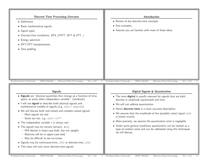
Discrete-Time Processing Overview Introduction • Review of key discrete-time concepts • Definitions • Few examples • Basic mathematical signals • Assume you are familiar with most of these ideas • Signal types • Discrete-time transforms: DFS, DTFT, DFT & FFT, z • Energy spectrum • DFT/FFT Interpretations • Zero padding Portland State University ECE 538/638 Discrete-Time Processing Ver. 1.10 1 Portland State University ECE 538/638 Discrete-Time Processing Ver. 1.10 2 Signals Digital Signals & Quantization • Signals are “physical quantities that change as a function of time, • The term digital is usually reserved for signals that are both space, or some other independent variable.” (textbook) discrete in amplitude (quantized) and time • I will use signal to describe both physical signals and • We will not address quantization mathematical models of signals (e.g. x ( n ) = cos( ωn ) ). • Hence discrete-time is a more accurate description • We will discuss both real-valued and complex-valued signals • We assume that the amplitude of the (possibly noisy) signal x ( n ) – Most signals are real is known exactly – Some are not: e.g. x ( n ) = e jωn • More precisely, we assume the quantization error is negligible • The independent variable n is always real • Under some general conditions quantization can be treated as a • The signals may be vectors (arrays): x ( n ) type of random noise and can be addressed using the techniques – Will denote in lower-case bold, but not upright we will discuss – Matrices will be in upper-case bold – May be difficult to see on-screen • Signals may be continuous-time, x ( t ) , or discrete-time, x ( n ) • This class will only cover discrete-time signals Portland State University ECE 538/638 Discrete-Time Processing Ver. 1.10 3 Portland State University ECE 538/638 Discrete-Time Processing Ver. 1.10 4

Signal Models Signal Classes There are two broad classes of signals • Signals recorded from natural phenomena have no precise mathematical description • Deterministic: Any signal that can be described by a • Mathematical analysis requires a precise mathematical description mathematical relationship is called – For example: x ( n ) = sin( ωn ) • To reconcile, we use models – The models are not exact • Random: signals that cannot be described accurately by a mathematical relationship – But are mathematically useful – For example: x ( n ) independently, identically distributed – Enable us to solve approximate problems exactly (i.i.d.), x ( n ) ∼ N (0 , 1) • We will focus on deterministic signals and systems first • These will be useful building blocks for describing the properties of random signals Portland State University ECE 538/638 Discrete-Time Processing Ver. 1.10 5 Portland State University ECE 538/638 Discrete-Time Processing Ver. 1.10 6 Discrete-Time Unit Impulse Discrete-Time Unit Step 1 1 n n 0 0 The discrete-time unit impulse is defined as The discrete-time unit step is defined as � � 0 , n � = 0 0 , n < 0 δ ( n ) = u ( n ) = 1 , n = 0 1 , n ≥ 0 • Sometimes called the unit sample • Also called the Kroneker delta • Note that δ ( n ) is an even function so δ ( n ) = δ ( − n ) Portland State University ECE 538/638 Discrete-Time Processing Ver. 1.10 7 Portland State University ECE 538/638 Discrete-Time Processing Ver. 1.10 8

Discrete-Time Unit Ramp Discrete-Time Basis Functions • There is a close relationship between δ ( n ) , u ( n ) and r ( n ) 4 δ ( n ) = u ( n ) − u ( n − 1) u ( n ) = r ( n + 1) − r ( n ) n n − 1 n 0 � � u ( n ) = δ ( k ) r ( n ) = u ( k ) The discrete-time unit ramp is defined as k = −∞ k = −∞ ∞ ∞ � � � u ( n ) = δ ( n − k ) r ( n ) = u ( n − 1 − k ) 0 , n < 0 r ( n ) = n u ( n ) = k =0 k =0 n, n ≥ 0 • The unit impulse can be used to sample a discrete-time signal x ( n ) : ∞ ∞ � � x (0) = x ( k ) δ ( k ) x ( n ) = x ( k ) δ ( n − k ) k = −∞ k = −∞ • This ability to use the unit impulse to extract a single value of x ( n ) is the basis of discrete-time convolution Portland State University ECE 538/638 Discrete-Time Processing Ver. 1.10 9 Portland State University ECE 538/638 Discrete-Time Processing Ver. 1.10 10 Example 1: 0 . 8 n and 0 . 8 − n Exponential Sequence The discrete-time exponential sequence is defined as 10 x ( n ) = a n If a is complex, 5 a = r e jω then x ( n ) is a complex-valued signal and may be written as 0 −10 −5 0 5 10 15 20 25 30 x ( n ) = r n e jωn = x R ( n ) + jx I ( n ) 1000 Recall Euler’s identity e jωn = cos( ωn ) + j sin( ωn ) 500 Thus x R ( n ) = r n cos( ωn ) x I ( n ) = r n sin( ωn ) 0 −10 −5 0 5 10 15 20 25 30 Time (n) Portland State University ECE 538/638 Discrete-Time Processing Ver. 1.10 11 Portland State University ECE 538/638 Discrete-Time Processing Ver. 1.10 12

Example 2: ( − 0 . 8) n and ( − 0 . 8) − n Example 1: MATLAB Code n = -10:30; % Time index 10 a = 0.8; subplot(2,1,1); 5 y = a.^(n); % Growing exponential h = stem(n,y); 0 set(h(1),’Marker’,’.’); set(gca,’Box’,’Off’); subplot(2,1,2); −5 y = a.^(-n); % Decaying exponential h = stem(n,y); −10 set(h(1),’Marker’,’.’); −10 −5 0 5 10 15 20 25 30 set(gca,’Box’,’Off’); xlabel(’Time (n)’); 1000 500 0 −500 −1000 −10 −5 0 5 10 15 20 25 30 Time (n) Portland State University ECE 538/638 Discrete-Time Processing Ver. 1.10 13 Portland State University ECE 538/638 Discrete-Time Processing Ver. 1.10 14 Example 2: MATLAB Code Example 3: e j 0 . 2 n n = -10:30; % Time index 1 a = 0.8; subplot(2,1,1); 0.5 y = (-a).^(n); % Growing exponential Real Part h = stem(n,y); 0 set(h(1),’Marker’,’.’); set(gca,’Box’,’Off’); −0.5 subplot(2,1,2); y = (-a).^(-n); % Decaying exponential −1 h = stem(n,y); −10 −5 0 5 10 15 20 25 30 35 40 set(h(1),’Marker’,’.’); set(gca,’Box’,’Off’); xlabel(’Time (n)’); 1 Imaginary Part 0.5 0 −0.5 −1 −10 −5 0 5 10 15 20 25 30 35 40 Time (n) Portland State University ECE 538/638 Discrete-Time Processing Ver. 1.10 15 Portland State University ECE 538/638 Discrete-Time Processing Ver. 1.10 16

Example 3: MATLAB Code Example 4: e j 0 . 2 n n = -10:40; % Time index Complex:Blue Real:Red Imaginary:Green N = length(n); w = 0.2; y = exp(j*w*n); subplot(2,1,1); h = stem(n,real(y)); set(h(1),’Marker’,’.’); 1 box off; grid on; ylim([-1.1 1.1]); 0.5 ylabel(’Real Part’); subplot(2,1,2); Real Part h = stem(n,imag(y)); 0 set(h(1),’Marker’,’.’); box off; grid on; −0.5 ylim([-1.1 1.1]); xlabel(’Time (n)’); 1 ylabel(’Imaginary Part’); −1 0 −10 0 10 20 30 −1 40 Imaginary Part Portland State University ECE 538/638 Discrete-Time Processing Ver. 1.10 17 Portland State University ECE 538/638 Discrete-Time Processing Ver. 1.10 18 Example 4: MATLAB Code Example 5: 0 . 95 ± n e j 0 . 5 n h = plot3(n,zeros(1,N),zeros(1,N),’k’); 1 hold on; h = plot3(ones(2,1)*n,[zeros(1,N);imag(y)],[zeros(1,N);real(y)],’b’); 0.5 h = plot3(n,imag(y),real(y),’b.’); Real Part h = plot3(ones(2,1)*n,1.1*ones(2,N),[zeros(1,N);real(y)],’r’); 0 h = plot3(n,1.1*ones(1,N),real(y),’r.’); h = plot3(ones(2,1)*n,[zeros(1,N);imag(y)],-1.1*ones(2,N),’g’); −0.5 h = plot3(n,imag(y),-1.1*ones(size(n)),’g.’); hold off; −1 grid on; −30 −20 −10 0 10 20 30 ylabel(’Imaginary Part’); zlabel(’Real Part’); title(’Complex:Blue Real:Red Imaginary:Green’); 1 axis([min(n) max(n) -1.1 1.1 -1.1 1.1]); view(27.5,22); 0.5 Real Part 0 −0.5 −1 −30 −20 −10 0 10 20 30 Time (n) Portland State University ECE 538/638 Discrete-Time Processing Ver. 1.10 19 Portland State University ECE 538/638 Discrete-Time Processing Ver. 1.10 20