Definitions and Examples I (10.1) Definitions and Examples I (10.1) - PowerPoint PPT Presentation
Outline: Chapter 10 Stochastic Processes 2 Definitions and Examples (10.1) D fi i i d E l (10 1) Types of Stochastic Processes (10.2) 204312 PROBABILITY AND 204312 PROBABILITY AND Random Variables from Random Processes RANDOM
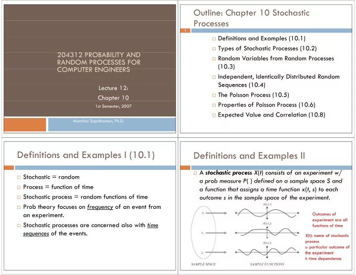
Outline: Chapter 10 Stochastic Processes 2 � Definitions and Examples (10.1) D fi i i d E l (10 1) � Types of Stochastic Processes (10.2) 204312 PROBABILITY AND 204312 PROBABILITY AND � Random Variables from Random Processes RANDOM PROCESSES FOR (10.3) ( 0 3) COMPUTER ENGINEERS COMPUTER ENGINEERS � Independent, Identically Distributed Random Sequences (10 4) Sequences (10.4) Lecture 12: � The Poisson Process (10.5) Chapter 10 p � Properties of Poisson Process (10.6) 1st Semester, 2007 � Expected Value and Correlation (10.8) p ( ) Monchai Sopitkamon, Ph.D. Definitions and Examples I (10.1) Definitions and Examples I (10.1) Definitions and Examples II Definitions and Examples II � A stochastic process X ( t ) consists of an experiment w/ � A stochastic process X ( t ) consists of an experiment w/ � Stochastic = random a prob measure P ( ) defined on a sample space S and � Process = function of time a function that assigns a time function x ( t , s ) to each a function that assigns a time function x ( t s ) to each � Stochastic process = random functions of time outcome s in the sample space of the experiment . � Prob theory focuses on frequency of an event from � P b th f f f t f an experiment. Outcomes of experiment are all p � Stochastic processes are concerned also with time functions of time sequences of the events. X ( t ): name of stochastic process s : particular outcome of the experiment the experiment t : time dependence
Definitions and Examples III Definitions and Examples III Definitions and Examples IV Definitions and Examples IV � Sample Function : A sample function x ( t , s ) is the time � Ex.10.1: Starting at launch time t = 0, X (t ) = temp in ° K on space shuttle’s surface. With each launch s , function associated with outcome s of an experiment . we record a temp sequence x ( t , s ). The ensemble of � A sample function corresponds to an outcome of a the experiment can be viewed as a group of the stochastic process experiment. p p possible temp sequences. For example, � Ensemble : The ensemble of a stochastic process is the x (8073.68, 175) = 207 (8073 68, 75) 07 set of all possible time functions that can result from set of all possible time functions that can result from 174 th an experiment . t s temp 207 means in the 175 th launch, i th 175 th l h 175 th t = 8073.68 the temp at t = 8073.68 sec after this launch is 207 ° K 176 th Definitions and Examples V Definitions and Examples V Definitions and Examples VI Definitions and Examples VI � Since the stochastic process produces two-dimensional sample � Since the stochastic process produces two-dimensional sample � Ex.10.4: An experiment where we record M ( t ), the no of 0 4 A h d M ( ) h f functions, there are two types of averages active calls at a phone switch at time t , at each second � Ensemble average : taken at t = t 0 , X ( t 0 ) is a RV, and we have the over an interval of 15 min. One trial of experiment over an interval of 15 min One trial of experiment averages (expected value and variance) that we studied before averages (expected value and variance) that we studied before yields sample fn m ( t , s ) shown in the fig. Each � Time average of a specific sample function: applied to a specific sample function, x ( t , s 0 ), and gives a number for this sample function. experiment performed yields some other fn m ( t , s ). This p p y ( , ) � Ex.10.2: From Ex.10.1, over all possible launches (s ) , the avg temp fn depends on the no of calls at the start of the after 8073.68 sec is E ( X (8073.68)) = 217 ° K ( ensemble avg ). In the 175 th launch, the avg temp over that space shuttle mission is observation period, the arrival times of new calls, and the duration of each call. An ensemble average is the 1 ∫ 671208.3 = ° avg no of calls in progress at t = 403 sec. A time avg is 175 th ( ,175) 187.43 x t dt K 671208.3 0 the avg no of calls in progress during a certain 15 min the avg no of calls in progress during a certain 15-min t interval. where the integral limit 671208.3 is the duration in sec of the shuttle mission. Time average Time a erage
Definitions and Examples V Definitions and Examples V Definitions and Examples VI Definitions and Examples VI � RVs that make up sample function m ( t , s ) include: RV h k l f i ( t ) i l d � m (0, s ): the no of ongoing calls at the start of experiment � X � X 1 , …, X m (0, s ) : the remaining time in sec of each of the m (0, X : the remaining time in sec of each of the m (0 s ) ongoing calls � N : the no of new calls that arrive during the experiment � S 1 , …, S N : the arrival times in sec of the N new calls � Y 1 , …, Y N : the calls durations in sec of each of the N new calls calls � X 1 , . . . , X N : the interarrival times of the N new arrivals � H , the number of calls that hang up during the experiment � D 1 , . . . , D H : the call completion times of the H calls that Figure 10.2 (p. 356) hang up A sample function m ( t,s ) of the random process M ( t ) described in Example 10.4. p ( , ) p ( ) p Types of Stochastic Processes I (10.2) Types of Stochastic Processes I (10.2) Types of Stochastic Processes II Types of Stochastic Processes II � Discrete-Value and Continuous-Value Processes Brownian Motion � X ( t ) is a discrete-value process if the set of all possible Process values of X ( t ) at all times t is a countable set S X ; otherwise X ( t ) is a continuous-value process . � Discrete-Time and Continuous-Time Processes � X ( t ) is a discrete-time process if X ( t ) is defined only for ( ) p ( ) y P i Poisson Process P a set of time instants; t n = nT , where T is a constant and n is an integer; otherwise X ( t ) is a continuous-time process . Sample functions of four kinds of stochastic processes. X cc ( t ) is a continuous-time, continuous-value process. X dc ( t ) is discrete-time, continuous-value process obtained by sampling X cc ( t ) every 0.1 seconds. Rounding X cc ( t ) to the nearest integer yields X cd ( t ), a continuous-time, discrete-value process. Lastly, X dd ( t ), a discrete-time, discrete-value process, can be obtained either by sampling X cd ( t ) or by rounding X dc ( t ).
Types of Stochastic Processes IV Types of Stochastic Processes IV Types of Stochastic Processes III Types of Stochastic Processes III 14 � From the previous fig., for a discrete-time process, the h f f d h W We obtain a continuous time, continuous valued b l d a) sample function is completely described by the ordered process when we record the temperature as a sequence of RVs X n = X ( nT ). sequence of RVs X = X ( nT ) continuous waveform over time continuous waveform over time � Random Sequence If at every moment in time, we round the temperature b) to the nearest degree then we obtain a continuous to the nearest degree, then we obtain a continuous � A random sequence X n is an ordered sequence of RVs X 0 , � A random sequence X is an ordered sequence of RVs X time, discrete valued process X 1 , … � Quiz10.2: For the temperature measurements of � Quiz10.2: For the temperature measurements of If we sample the process in part (a) every T seconds, If we sample the process in part (a) every T seconds c) c) Ex.10.3, construct examples of the measurement process then we obtain a discrete time, continuous valued such that the process is either process Discrete-time, discrete-value Rounding the samples in part (c) to the nearest integer a) d) Discrete-time, continuous-value degree yields a discrete time, discrete valued process. b) Continuous-time, discrete-value c) Continuous-time, continuous-value d) Random Variables from Random Processes I Random Variables from Random Processes (10.3) II � Ex.10.8: Suppose that at time instants T = 0, 1, 2, 0 8 S 0 2 � We use X ( t 1 ) to represent a RV whose sample value …, we roll a die and record the outcome N T where is x ( t 1 , s ), which is a sample fn x ( t , s ) at particular 1 ≤ N T ≤ 6. We then define the random process 1 ≤ N ≤ 6 W th d fi th d time instant t 1 and sequence s . X ( t ) such that for T ≤ t ≤ T + 1, X ( t ) = N T . In this � However, X ( t ) can refer to either the random process , ( ) p case the experiment consists of an infinite sequence case, the experiment consists of an infinite sequence or the RV that corresponds to the value of the of rolls and a sample fn is just the waveform random process at time t . random process at time t . corresponding to the particular sequence of rolls corresponding to the particular sequence of rolls. What is the PMF of X (3.5) ? � If X ( t 1 ) is a discrete RV, it has a PMF ( ) ( ) P x X t 1 The RV X (3.5) is the value of the die roll at time 3. The RV X (3.5) is the value of the die roll at time 3. � If X ( t 1 ) is a continuous RV, it has a PDF If X ( ) i i RV i h PDF ( ) ( ) ( ) f f x X t = ⎧ 1 1/ 6 1,...,6, x = ⎨ ( ) P x X (3.5) (3.5) ⎩ ⎩ 0 0 otherwise th i (3.5) ( ) = prob that X = x ( x = 1, …, 6) at time t = 3 P x X
Recommend
More recommend
Explore More Topics
Stay informed with curated content and fresh updates.
