Towards an information-theoretic model of the Allison mixture A - PowerPoint PPT Presentation
Lachlan J. Gunn 1 Franois Chapeau-Blondeau 2 Andrew Allison 1 Derek Abbott 1 1 School of Electrical and Electronic Engineering The University of Adelaide 2 Laboratoire Angevin de Recherche en Ingnierie des Systmes (LARIS) University of
Lachlan J. Gunn 1 François Chapeau-Blondeau 2 Andrew Allison 1 Derek Abbott 1 1 School of Electrical and Electronic Engineering The University of Adelaide 2 Laboratoire Angevin de Recherche en Ingénierie des Systèmes (LARIS) University of Angers Towards an information-theoretic model of the Allison mixture A canonical measure of dependence for a special mixture distribution
Mixture processes subsystems. ▶ Many systems can be split into independent multiplexed X ₁ Y X ₂ S X ₂ X ₁ ▶ These situations occur quite often.
Applications of mixture processes Yunhan Dong, DSTO-RR-0316 “Distribution of X-Band High Resolution and High Grazing Angle Sea Clutter” (2006) ▶ Radar—sea clutter can be modelled with a KK-distribution p KK (x) = (1 − k) p K (x; ν₁ , σ₁ ) + k p K (x; ν₂ , σ₂ ) Photo: Malene Thyssen Photo: Graham Horn Rolling sea (1 − k) of …and an occasional the time… spike in the return.
Applications of mixture processes Gales, Young, “The Application of Hidden Markov Models in Speech Recognition,’, Foundations and Trends in Signal Processing, 1 (3), 2007. to form the sound of words. ▶ Speech—random signals corresponding to phenomes are joined Nasal Cavity Image: doi:10.3389/fnhum.2013.00749 Palate (Roof of Mouth) Velum Alveolar "bat" Ridge Oral Cavity Lips Teeth Voice Box Tongue (Tongue tip & Tongue Blade) Image: Tavin, Wikimedia /b/ Commons /æ/ /t/ Photo: Oren Peles
Applications of mixture processes be modelled by a mixture of Poisson distributions. ▶ Natural language processing—word frequency distributions can Mentions of Javert in Les Misérables Javertiness Battle of Waterloo Javert Table of testifies contents Javert's Valjean's introduction monologue
The Allison Mixture ▶ Which input process is visible at the output? ▶ One option is to choose independently each time: p Y ( y ) = kp 0 ( y ) + ( 1 − k ) p 1 ( y ) = ⇒ Independent inputs yield independent outputs. ▶ This is too restrictive, often the choices of sample are dependent.
The Allison Mixture α₁ α₂ ▶ Instead, let’s—sometimes—switch from one input to the other. 1 −α₁ X ₁ X ₂ 1 −α₂ ▶ This forms a Markov chain.
Independence of the Allison mixture ▶ This makes output samples dependent, even if the inputs are not. X ₁ Y X ₂ S X ₂ X ₁
Autocovariance α 1 α 2 Gunn, Allison, Abbott, “Allison mixtures: where random digits obey thermodynamic principles”, International Journal of Modern Physics: Conference Series 33 (2014). ▶ It is known that the lag-one autocovariance is given by R YY [ 1 ] = ( 1 − α 1 − α 2 )( μ 1 − μ 2 ) 2 , α 1 + α 2 where μ 1 and μ 2 are the input means. ▶ If X 1 and X 2 are N ( μ i , σ 2 ) then this is just a noisy version of S.
Uncorrelatedness ▶ This gives us the conditions for a correlated output: α 1 ̸ = 0 α 2 ̸ = 0 α 1 + α 2 ̸ = 1 μ 1 ̸ = μ 2 ▶ If any of these are violated, consecutive samples are uncorrelated.
Moving beyond a single step in the Allison mixture. Let’s fill in the remaining details! α 2 α 1 Allison mixture—the choice of input is still Markovian. Gunn, Chapeau-Blondeau, Allison, Abbott, Unsolved Problems of Noise (2015). ▶ We previously demonstrated only the appearance of correlation ▶ The state-transition matrix of the Markov chain S is [ 1 − α 1 ] P = 1 − α 2 . ▶ Taking every k-th sample of an Allison mixture yields another
Moving beyond a single step k-step transition probabilities α 2 α 1 respectively. ▶ By taking P k and reading ofg the minor diagonal, we find the [ 1 − ( 1 − α 1 − α 2 ) k ] α 1 [ k ] = α 1 + α 2 [ 1 − ( 1 − α 1 − α 2 ) k ] α 2 [ k ] = . α 1 + α 2 ▶ The initial coeffjcients are the stationary probabilities π 1 and π 2
Multi-step autocovariance yielding α 1 α 2 ▶ We substitute these back into the autocovariance formula, R YY [ k ] = ( μ 1 − μ 2 ) 2 ( 1 − α 1 − α 2 ) k α 1 + α 2 = R YY [ 1 ]( 1 − α 1 − α 2 ) k . ▶ The autocovariance thus decays exponentially with time.
Autoinformation entropy rate. induce correlation. ▶ Autoinformation provides a more-easily-computed alternative to ▶ Information theory lets us capture dependence that does not
Autoinformation Definition (Autoinformation) which simplifies, for a stationary process, to We define the autoinformation I XX [ n , k ] I XX [ n , k ] = I ( X [ n ]; X [ n − k ]) , I XX [ k ] = H ( X [ n ] , X [ n − k ]) − 2H ( X [ n ]) .
A path towards Allison mixture autoinformation ▶ Can we take the same approach as with autocovariance? S[n] Calculate Calculate Autocovariance Autoinformation R ss [k] I ss [k] Transform according Transform according to input processes to input processes R ss [k] ( μ₁−μ₂ )² ???
α 2 Sampling process autoinformation α 1 (1) ▶ We compute the autoinformation from the stationary and transition probabilities using I ( X ; Y ) = H ( X ) − H ( X | Y ) . α 2 ( 1 − α 1 ) log 2 1 − α 1 I xx [ 1 ] = α 1 + α 2 α 1 ( 1 − α 2 ) log 2 1 − α 2 + α 1 + α 2 + log 2 ( α 1 + α 2 ) ,
Sampling process autoinformation α₂ α₁ Autoinformation 1.0 1.0 0.8 0.6 0.5 0.4 0.2 0.0 0.0 0.0 0.5 1.0
Sampling process autoinformation Autoinformation (bits) 10¯ ⁰ 10¯¹ 10¯² 10¯³ 10¯ ⁴ 10¯ ⁵ 0 5 10 15 20 Lag
Allison mixture autoinformation ▶ How do we apply this to the Allison mixture? ▶ Binary-valued outputs: X 1 [ k ] , X 2 [ k ] ∈ 0 , 1 ▶ Use Bayes law to find the probability of each state: P [ Y [ k ] | S [ k ] = s ] π s P [ S [ k ] = s | Y [ k ]] = ∑ q P [ Y [ k ] | S [ k ] = q ] π q ▶ We now know enough to find the transition probabilities for Y: Y [ k ] − → S [ k ] − → S [ k + 1 ] − → Y [ k + 1 ]
Allison mixture autoinformation with transition probabilities is not the end of the road. ▶ It turns out that the previous autoinformation formula works here α 1 ( 1 − p 0 ) [ p 0 ( 1 − α 0 ) + p 1 α 0 ] + α 0 ( 1 − p 1 ) [ p 0 α 1 + p 1 ( 1 − α 1 )] α ′ 0 = α 0 ( 1 − p 1 ) + α 1 ( 1 − p 0 ) α 1 p 0 [( 1 − p 0 )( 1 − α 0 ) + ( 1 − p 1 ) α 0 ] + α 0 p 1 [( 1 − p 0 ) α 1 + ( 1 − p 1 )( 1 − α 1 )] α ′ 1 = . α 0 p 1 + α 1 p 0 ▶ A formula of this complexity that only works for binary processes
Open problems processes? systems. ▶ Can a similar technique be applied to more general input ▶ Continuous distributions are important. ▶ Could this system be useful for studying transfer entropy? ▶ Transfer entropy is the “information transfer” between two ▶ Previous studies have revolved around chaotic systems.
Recommend
More recommend
Explore More Topics
Stay informed with curated content and fresh updates.

