Kalman Filters 1 Kalman filters Modelling systems described by a - PowerPoint PPT Presentation
Kalman Filters 1 Kalman filters Modelling systems described by a set of continuous variables, e.g., tracking a bird flying X t = X, Y, Z, X, Y , Z . Airplanes, robots, ecosystems, economies, chemical plants, planets, . . . X X t t
Kalman Filters 1
Kalman filters Modelling systems described by a set of continuous variables, e.g., tracking a bird flying— X t = X, Y, Z, ˙ X, ˙ Y , ˙ Z . Airplanes, robots, ecosystems, economies, chemical plants, planets, . . . X X t t +1 X X t t +1 Z Z t t +1 Gaussian prior, linear Gaussian transition model and sensor model 2
Updating Gaussian distributions Prediction step: if P ( X t | e 1: t ) is Gaussian, then prediction � P ( X t +1 | e 1: t ) = x t P ( X t +1 | x t ) P ( x t | e 1: t ) d x t is Gaussian. If P ( X t +1 | e 1: t ) is Gaussian, then the updated distribution P ( X t +1 | e 1: t +1 ) = α P ( e t +1 | X t +1 ) P ( X t +1 | e 1: t ) is Gaussian Hence P ( X t | e 1: t ) is multivariate Gaussian N ( µ t , Σ t ) for all t General (nonlinear, non-Gaussian) process: description of posterior grows unboundedly as t → ∞ 3
Simple 1-D example Gaussian random walk on X –axis, s.d. σ x , sensor s.d. σ z µ t +1 = ( σ 2 t + σ 2 x ) z t +1 + σ 2 t +1 = ( σ 2 t + σ 2 x ) σ 2 z µ t z σ 2 σ 2 t + σ 2 x + σ 2 σ 2 t + σ 2 x + σ 2 z z 0.45 0.4 0.35 P(x1 | z1=2.5) 0.3 0.25 P(x0) P(X) 0.2 0.15 0.1 P(x1) 0.05 0 * z1 -8 -6 -4 -2 0 2 4 6 8 X position 4
General Kalman update Transition and sensor models: P ( x t +1 | x t ) = N ( Fx t , Σ x )( x t +1 ) P ( z t | x t ) = N ( Hx t , Σ z )( z t ) F is the matrix for the transition; Σ x the transition noise covariance H is the matrix for the sensors; Σ z the sensor noise covariance Filter computes the following update: µ t +1 = F µ t + K t +1 ( z t +1 − HF µ t ) Σ t +1 = ( I − K t +1 )( FΣ t F ⊤ + Σ x ) where K t +1 = ( FΣ t F ⊤ + Σ x ) H ⊤ ( H ( FΣ t F ⊤ + Σ x ) H ⊤ + Σ z ) − 1 is the Kalman gain matrix Σ t and K t are independent of observation sequence, so compute offline 5
2-D tracking example: filtering 2D filtering 12 true observed filtered 11 10 9 Y 8 7 6 8 10 12 14 16 18 20 22 24 26 X 6
2-D tracking example: smoothing 2D smoothing 12 true observed smoothed 11 10 9 Y 8 7 6 8 10 12 14 16 18 20 22 24 26 X 7
Where it breaks Cannot be applied if the transition model is nonlinear Extended Kalman Filter models transition as locally linear around x t = µ t Fails if systems is locally unsmooth 8
Recommend
More recommend
Explore More Topics
Stay informed with curated content and fresh updates.
