The Dynamics of Star Cluster Formation Juan Pablo Farias Jonathan - PowerPoint PPT Presentation
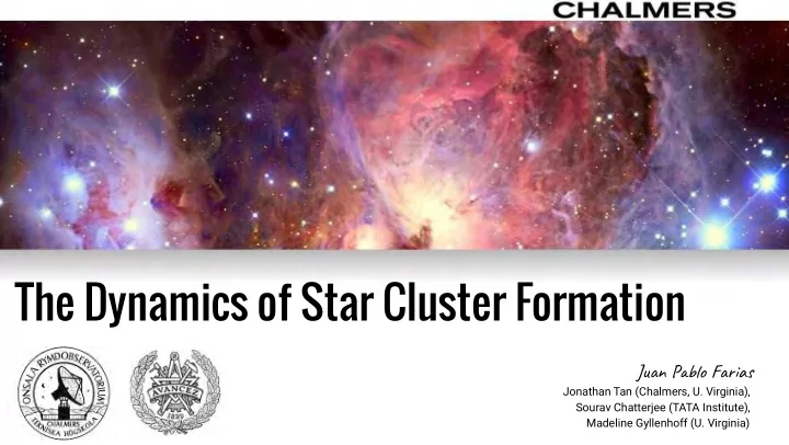
The Dynamics of Star Cluster Formation Juan Pablo Farias Jonathan Tan (Chalmers, U. Virginia), Sourav Chatterjee (TATA Institute), Madeline Gyllenhoff (U. Virginia) How is gas transformed into a star cluster? What is the star formation
The Dynamics of Star Cluster Formation Juan Pablo Farias Jonathan Tan (Chalmers, U. Virginia), Sourav Chatterjee (TATA Institute), Madeline Gyllenhoff (U. Virginia)
How is gas transformed into a star cluster? ● What is the star formation rate? (and its evolution) ● What is the primordial stellar population? Binary fraction and properties – Mass segregation – ● Can this population be signifjcantly processed during cluster formation?
What is the timescale of formation? ● Fast formation models: (e.g. Elmegreen 200,2007; Hartmann & Burkert 2007) ○ Short timescales ~1 or 2 free fall times ○ Cloud is collapsing quickly ● Slow formation models: (e.g. Tan, Krumholtz & Mckee 2006, Nakamura & Li 2007,2014) ○ several free fall times ○ cloud is in approximate equilibrium.
Dynamical Timescales It is important to note that star cluster’s dynamical evolution timescales scales with density Formation rate: ● Free fall time: “The time a cloud of gas need to collapse under its own weight if no forces support it” (Krumholtz & McKee 2005) Star formation effjciency per free fall time ● Crossing time: “The time a typical star in a star cluster needs to cross the system”
Stages of star cluster formation Hydrodynamics e.g. Nakamura & Li (2007,20014), Bate+(2005,2014),Wu+(2017,2018), e.g. Baumgardt & Kroupa (2007), Smith+(2011,2013), Farias et al. (2015) Proszkow & Adams(2009) Stellar Dynamics Stellar dynamics cons: Our Approach: ● ● Sink particles Study the formation stage from a ● Not so accurate N-body codes dynamical perspective. ● ● Small samples Make assumptions for the gas behaviour and star formation.
The Star Cluster formation model: l Gradual formation of Stars e d o M p (Farias, Tan, Chatterjee 2017,2019) m u l C Mckee & Tan (2003) e r o C t n e l u b r u T see estimates from DaRio+(2014) in the ONC Nbody6++SF ● 𝝑 fg = 0.01, 0.03, 0.1, 0.3, 1, ∞ Aarseth (2003), Wang+(2015), Farias+(2019) Uniform SFE ( = ● 𝝑 0.5 fjducial case) ● Stars follow the mass and velocity profjle of the parent clump ● Star cluster is isolated ● Gas is exhausted and expelled as the stars form ● Star formation rate is constant with time
Sample simulation: Fiducial case: ● Σ cl = 0.1 g cm -2 ● 50% binaries ● Stellar evolution 𝝑 fg = 0.03 ● ● 𝝑 = 0.5 Gas (shown as red area) decrease with time as stars are created according to the assumed star formation effjciency
Sample simulation: Fiducial case: ● Σ cl = 0.1 g cm -2 ● 50% binaries ● Stellar evolution 𝝑 fg = 0.03 ● ● 𝝑 = 0.5 Gas (shown as red area) decrease with time as stars are created according to the assumed star formation effjciency
Perturbing the Model: Elliptical Clouds A ONC = 2.0 (DaRio et al. 2014) ● Star clusters are do not form in spherical systems. Next Step: Perturbing the model .. ● Stretch it R Z A = Z R Madeline Gyllenhofg University of Virginia
Perturbing the Model: Elliptical Clouds Sample simulation: Fiducial case (instant. Formation): ● Σ cl = 0.1 g cm -2 ● 50% binaries ● Stellar evolution 𝝑 fg = 0.03 ● ● 𝝑 = 0.5 ● A i = 3
Perturbing the Model: Elliptical Clouds Sample simulation: Fiducial case (Gradual Formation): ● Σ cl = 0.1 g cm -2 ● 50% binaries ● Stellar evolution 𝝑 fg = 0.03 ● ● 𝝑 = 0.5 ● A i = 3
Perturbing the model: Turbulence ● Star clusters are do not form in spherical systems. Next Step: Perturbing the model .. ● Stretch it ● Apply turbulence
Perturbing the model: Turbulence ● Perturbing the model Turbulent background with Turbulent Core Scale free Turbulent the density and velocity Model Box Simulation profjle of the TCM
Perturbing the model: Turbulence ● Perturbing the model Turbulent background with Turbulent Core Scale free Turbulent the density and velocity Model Box Simulation profjle of the TCM
Results
Expansion Rates Mass segregation Results Relaxation timescales Stellar age gradients Bound Fractions Dynamical Ejections Velocity dispersion profiles Brown Dwarf distributions
Expansion Rates Mass segregation Results Relaxation timescales Stellar age gradients Bound Fractions Dynamical Ejections Velocity dispersion profiles Brown Dwarf distributions
Formation timescales: 𝝑 = 0.5 Number of Dynamical times 𝝑 ff 𝝑 ff /𝝑 Formation time (Myr) 0.01 50 0.03 16.6 0.1 5 0.3 1.6 1.0 0.5
Different formation timescales ● We test our fjducial model under difgerent values of 𝝑 fg . Number Density (stars/pc 3 ) ● Difgerent formation timescales defjnes how long number densities remains high slowest fastest The density starts low as there are less stars but raises and stays high for some “physical” time. But, how long is that time in crossing times?
Dynamical Ejections
Dynamical Ejections Low Density Case Probability Probability Velocity Energy slowest fastest
Dynamical Ejections ● We look for massive runaway stars at difgerent velocity cuts. Observations* ● Low forming clusters produce more runaway stars than fast forming clusters. * e.g. Gies 1987; Stone 1991; De Wit et al. 2005
Stellar Ages
Stellar Age gradients Getman et al. 2018 ● Observations suggest that star clusters tend to have positve age gradients (Getman et al 2018) ● i.e. In general, younger stars are in the center and older stars in the outskirts. Standardized ages and distances SfjNCs cluters MYStIX clusters (Getman et al. 2018) (Kuhn et al. 2014)
Stellar Age gradients ● Our methods enable us to study the evolution of stellar systems with difgerent stellar ages slowest fastest Standardized ages and distances
Stellar Age gradients ● Our methods enable us to study the evolution of stellar systems with difgerent stellar ages slowest Standardized ages and distances fastest
Stellar Age gradients ● Our methods enable us to study the evolution of stellar systems with difgerent stellar ages slowest Standardized ages and distances fastest
Brown Dwarfs
Brown Dwarfs Slopes
Summary and Future Work ● The formation of a cluster may take several dynamical times, and considerable dynamical processing may happen during formation. ● Longer formation time increases chances for energetic dynamical ejections. ● We have developed a method for testing any star cluster formation model from the Stellar Dynamics perspective. ● Next steps: Test the consequences of the difgerent levels of In the models substructure in the stellar population dynamics. Include the ability of using an arbitrary In the code background potential in Nbody6++SF. Compute synthetic observation in order to In the analysis compare our models with the JWST and Gaia.
Recommend
More recommend
Explore More Topics
Stay informed with curated content and fresh updates.
