Dynamical Systems in Gene Regulation Peter Schuster Institut fr - PowerPoint PPT Presentation
Dynamical Systems in Gene Regulation Peter Schuster Institut fr Theoretische Chemie, Universitt Wien, Austria and The Santa Fe Institute, Santa Fe, New Mexico, USA Jozef Stefan Institute Ljubljana, 10.02.2006 Web-Page for further
Dynamical Systems in Gene Regulation Peter Schuster Institut für Theoretische Chemie, Universität Wien, Austria and The Santa Fe Institute, Santa Fe, New Mexico, USA Jozef Stefan Institute Ljubljana, 10.02.2006
Web-Page for further information: http://www.tbi.univie.ac.at/~pks
1. Forward and inverse problems in reaction kinetics 2. Reverse engineering – A simple example 3. A glimpse of regulation kinetics 4. Genetic and metabolic networks – MiniCellSim 5. How do model metabolisms evolve?
1. Forward and inverse problems in reaction kinetics 2. Reverse engineering – A simple example 3. A glimpse of regulation kinetics 4. Genetic and metabolic networks – MiniCellSim 5. How do model metabolisms evolve?
Kinetic differential equations d x = = = ( ; ) ; ( , , ) ; ( , , ) K K f x k x x x k k k 1 1 n m d t Reaction diffusion equations ∂ x = ∇ + 2 ( ; ) Solution curves : ( ) D x f x k x t ∂ t x i (t) Concentration Parameter set = ( T , p , p H , I , ) ; j 1 , 2 , , m K K k j General conditions : T , p , pH , I , ... t ( 0 ) Initial conditions : x Time Boundary conditions : � boundary ... S , normal unit vector ... u x S = Dirichlet : ( , ) g r t ∂ S = x = ⋅ ∇ ˆ Neumann : ( , ) u x g r t ∂ u The forward problem of chemical reaction kinetics (Level I)
Kinetic differential equations d x = = = ( ; ) ; ( , , ) ; ( , , ) K K f x k x x x k k k 1 1 n m d t Reaction diffusion equations ∂ x 2 = ∇ + Genome: Sequence I G ( ; ) Solution curves : ( ) D x f x k x t ∂ t x i (t) Concentration Parameter set = ( G I ; , , , , ) ; 1 , 2 , , K K k j T p p H I j m General conditions : T , p , pH , I , ... t ( 0 ) Initial conditions : x Time Boundary conditions : boundary ... S , normal unit vector � ... u x S = Dirichlet : ( , ) g r t ∂ S = x = ⋅ ∇ ˆ ( , ) Neumann : u x g r t ∂ u The forward problem of biochemical reaction kinetics (Level I)
Kinetic differential equations d x = = = ( ; ) ; ( , , ) ; ( , , ) K K f x k x x x k k k 1 1 n m d t Reaction diffusion equations ∂ x = ∇ + 2 ( ; ) D x f x k ∂ t General conditions : T , p , pH , I , ... ( 0 ) Initial conditions : x Genome: Sequence I G Boundary conditions : boundary ... S , normal unit vector � ... u Parameter set x S = = Dirichlet : ( , ) ( G I ; , , , , ) ; 1 , 2 , , g r t K K k j T p p H I j m ∂ S = x = ⋅ ∇ Neumann : ˆ ( , ) u x g r t ∂ u Data from measurements (t ); = 1, 2, ... , x j N j x i (t ) j Concentration The inverse problem of biochemical t Time reaction kinetics (Level I)
Kinetic differential equations d x = = = f ( ; ) ; ( , , ) ; ( , , ) K K x k x x x k k k 1 1 n m d t Bifurcation analysis Reaction diffusion equations � ( , ; ) ∂ k k j k i x = ∇ 2 + f ( ; ) Genome: Sequence I G D x x k ∂ t k i P x n P Parameter set x n P x m = ( G I ; , , , , ) ; 1 , 2 , , K K k j T p p H I j m x m ( ) x t General conditions : T , p , pH , I , ... P time ( 0 ) Initial conditions : x x n x m k j Boundary conditions : boundary ... S , normal unit vector � ... u x S = Dirichlet : ( , ) g r t ∂ S = x = ⋅ ∇ ˆ Neumann : ( , ) u x g r t ∂ u The forward problem of bifurcation analysis (Level II)
Kinetic differential equations d x = = = ( ; ) ; ( , , ) ; ( , , ) f x k x x K x k k K k 1 1 n m d t Reaction diffusion equations ∂ x = ∇ + 2 ( ; ) D x f x k ∂ t General conditions : T , p , pH , I , ... ( 0 ) Initial conditions : x Genome: Sequence I G Boundary conditions : � boundary ... S , normal unit vector ... u Parameter set x S = = Dirichlet : ( , ) ( G I ; , , , , ) ; 1 , 2 , , g r t K K k j T p p H I j m ∂ S = x Neumann : = ⋅ ∇ ˆ ( , ) u x g r t ∂ u Bifurcation pattern � ( , ; ) k k j k i k 2 P 1 x n P 2 x P x m x The inverse problem of bifurcation P analysis (Level II) x k 1 x
1. Forward and inverse problems in reaction kinetics 2. Reverse engineering – A simple example 3. A glimpse of regulation kinetics 4. Genetic and metabolic networks – MiniCellSim 5. How do model metabolisms evolve?
Stock Solution [A] = a Reaction Mixture [A],[X] 0 r * A k 1 A X X A A A X A A k 2 A X A X k 3 A A +2 3 X A X X k 4 A A � R- A r X 1 Flow rate = A r A A 0 A X A X A X r 0 X X X X A A
0.5 � r Stationary concentration x Thermodynamic 0.4 branch 0.3 0.2 Bistability r cr,1 r cr,2 0.1 0.02 0.04 0.06 0.08 0.10 0.12 0.14 Flow rate r
r Kinetic differential equations: * A d [ A ] d a = = − − + 2 + + 2 ( ) ( ) ( ) r a a k k x a k k x x 0 1 3 2 4 d t d t k 1 d [ X ] d x A X = = − + + − + 2 2 ( ) ( ) r x k k x a k k x x 1 3 2 4 k 2 d t d t k 3 +2 3 A X X k 4 r 0 A r 0 X
r Kinetic differential equations: * A d [ A ] d a = = − − + 2 + + 2 ( ) ( ) ( ) r a a k k x a k k x x 0 1 3 2 4 d t d t k 1 d [ X ] d x A X = = − + + − + 2 2 ( ) ( ) r x k k x a k k x x 1 3 2 4 k 2 d t d t k 3 Steady states: +2 3 A X X + − + + + − = 3 2 k 4 ( ) ( ) 0 x k k x k a x k k r k a 3 4 3 0 1 2 1 0 r 0 A r 0 X
r Kinetic differential equations: * A d [ A ] d a = = − − + 2 + + 2 ( ) ( ) ( ) r a a k k x a k k x x 0 1 3 2 4 d t d t k 1 d [ X ] d x A X = = − + + − + 2 2 ( ) ( ) r x k k x a k k x x 1 3 2 4 k 2 d t d t k 3 Steady states: +2 3 A X X + − + + + − = 3 2 k 4 ( ) ( ) 0 x k k x k a x k k r k a 3 4 3 0 1 2 1 0 r = = α = = − + + α − α = 3 2 , 1 : 2 ( 2 ) 0 k k k k x x a x r a 0 A 1 2 3 4 0 0 r 0 X
r Kinetic differential equations: * A d [ A ] d a = = − − + 2 + + 2 ( ) ( ) ( ) r a a k k x a k k x x 0 1 3 2 4 d t d t k 1 d [ X ] d x A X = = − + + − + 2 2 ( ) ( ) r x k k x a k k x x 1 3 2 4 k 2 d t d t k 3 Steady states: +2 3 A X X + − + + + − = 3 2 k 4 ( ) ( ) 0 x k k x k a x k k r k a 3 4 3 0 1 2 1 0 r = = α = = − + + α − α = 3 2 , 1 : 2 ( 2 ) 0 k k k k x x a x r a 0 A 1 2 3 4 0 0 Polynomial discriminant of the cubic equation: r 2 α 4 a a 2 2 = + α − + α − α + α + α + = 3 2 2 3 2 216 D ( 6 0 ) ( 12 5 ) 8 4 0 0 0 r r r a a X 0 0 8 2
r Kinetic differential equations: * A d [ A ] d a = = − − + 2 + + 2 ( ) ( ) ( ) r a a k k x a k k x x 0 1 3 2 4 d t d t k 1 d [ X ] d x A X = = − + + − + 2 2 ( ) ( ) r x k k x a k k x x 1 3 2 4 k 2 d t d t k 3 Steady states: +2 3 A X X + − + + + − = 3 2 k 4 ( ) ( ) 0 x k k x k a x k k r k a 3 4 3 0 1 2 1 0 r = = α = = − + + α − α = 3 2 , 1 : 2 ( 2 ) 0 k k k k x x a x r a 0 A 1 2 3 4 0 0 Polynomial discriminant of the cubic equation: r 2 α 4 a a 2 2 = + α − + α − α + α + α + = 3 2 2 3 2 216 D ( 6 0 ) ( 12 5 ) 8 4 0 0 0 r r r a a X 0 0 8 2 � � D < 0 : 3 roots r , r , and r , 2 are positive r = r - r 1 2 3 1 2
0.6 0.00 0.4 � r 0.2 0.01 0.0 � 2.5 0.02 2.0 1.5 a 0 1.0 0.03 0.5 Range of hysteresis as a function of the parameters a 0 and �
1. Forward and inverse problems in reaction kinetics 2. Reverse engineering – A simple example 3. A glimpse of regulation kinetics 4. Genetic and metabolic networks – MiniCellSim 5. How do model metabolisms evolve?
Active states of gene regulation
Promotor III State : inactive state Repressor Activator binding site RNA polymerase Promotor III State : inactive state Activator Repressor RNA polymerase Inactive states of gene regulation
Cross-regulation of two genes
n p = Activation : ( ) j F p + n i j K p j K = Repression : ( ) F p + n i j K p j = , 1 , 2 i j Gene regulatory binding functions
Recommend
More recommend
Explore More Topics
Stay informed with curated content and fresh updates.
