The Bernoulli Generalized Likelihood Ratio test (BGLR) for - PowerPoint PPT Presentation
The Bernoulli Generalized Likelihood Ratio test (BGLR) for Non-Stationary Multi-Armed Bandits Research Seminar at PANAMA, IRISA lab, Rennes Lilian Besson PhD Student SCEE team, IETR laboratory, CentraleSuplec in Rennes & SequeL team,
The Bernoulli Generalized Likelihood Ratio test (BGLR) for Non-Stationary Multi-Armed Bandits Research Seminar at PANAMA, IRISA lab, Rennes Lilian Besson PhD Student SCEE team, IETR laboratory, CentraleSupélec in Rennes & SequeL team, CRIStAL laboratory, Inria in Lille Thursday 6 th of June, 2019
Publications associated with this talk Joint work with my advisor Émilie Kaufmann : “Analyse non asymptotique d’un test séquentiel de détection de ruptures et application aux bandits non stationnaires” by Lilian Besson & Émilie Kaufmann → presented at GRETSI , in Lille (France), next August 2019 ֒ ֒ → perso.crans.org/besson/articles/BK__GRETSI_2019.pdf “The Generalized Likelihood Ratio Test meets klUCB: an Improved Algorithm for Piece-Wise Non-Stationary Bandits” by Lilian Besson & Émilie Kaufmann Pre-print on HAL-02006471 and arXiv:1902.01575 Thursday 6 th of June, 2019 Lilian Besson BGLR test and Non-Stationary MAB 2 / 47
Outline of the talk Outline of the talk 1 (Stationary) Multi-armed bandits problems 2 Piece-wise stationary multi-armed bandits problems 3 The BGLR test and its finite time properties 4 The BGLR-T + klUCB algorithm 5 Regret analysis 6 Numerical simulations Thursday 6 th of June, 2019 Lilian Besson BGLR test and Non-Stationary MAB 3 / 47
1. (Stationary) Multi-armed bandits problems 1. (Stationary) Multi-armed bandits problems 1 (Stationary) Multi-armed bandits problems 2 Piece-wise stationary multi-armed bandits problems 3 The BGLR test and its finite time properties 4 The BGLR-T + klUCB algorithm 5 Regret analysis 6 Numerical simulations Thursday 6 th of June, 2019 Lilian Besson BGLR test and Non-Stationary MAB 4 / 47
1. (Stationary) Multi-armed bandits problems What is a bandit problem? Multi-armed bandits = Sequential decision making problems in uncertain environments : → Interactive demo perso.crans.org/besson/phd/MAB_interactive_demo/ ֒ Ref: [Bandits Algorithms, Lattimore & Szepesvári, 2019], on tor-lattimore.com/downloads/book/book.pdf Thursday 6 th of June, 2019 Lilian Besson BGLR test and Non-Stationary MAB 5 / 47
1. (Stationary) Multi-armed bandits problems Mathematical model Mathematical model Discrete time steps t = 1 , . . . , T The horizon T is fixed and usually unknown At time t , an agent plays the arm A ( t ) ∈ { 1 , . . . , K } , then she observes the iid random reward r ( t ) ∼ ν k , r ( t ) ∈ R Thursday 6 th of June, 2019 Lilian Besson BGLR test and Non-Stationary MAB 6 / 47
1. (Stationary) Multi-armed bandits problems Mathematical model Mathematical model Discrete time steps t = 1 , . . . , T The horizon T is fixed and usually unknown At time t , an agent plays the arm A ( t ) ∈ { 1 , . . . , K } , then she observes the iid random reward r ( t ) ∼ ν k , r ( t ) ∈ R Usually, we focus on Bernoulli arms ν k = Bernoulli( µ k ) , of mean µ k ∈ [0 , 1] , giving binary rewards r ( t ) ∈ { 0 , 1 } . Thursday 6 th of June, 2019 Lilian Besson BGLR test and Non-Stationary MAB 6 / 47
1. (Stationary) Multi-armed bandits problems Mathematical model Mathematical model Discrete time steps t = 1 , . . . , T The horizon T is fixed and usually unknown At time t , an agent plays the arm A ( t ) ∈ { 1 , . . . , K } , then she observes the iid random reward r ( t ) ∼ ν k , r ( t ) ∈ R Usually, we focus on Bernoulli arms ν k = Bernoulli( µ k ) , of mean µ k ∈ [0 , 1] , giving binary rewards r ( t ) ∈ { 0 , 1 } . � T Goal : maximize the sum of rewards r ( t ) t =1 � � � T or maximize the sum of expected rewards E r ( t ) t =1 Thursday 6 th of June, 2019 Lilian Besson BGLR test and Non-Stationary MAB 6 / 47
1. (Stationary) Multi-armed bandits problems Mathematical model Mathematical model Discrete time steps t = 1 , . . . , T The horizon T is fixed and usually unknown At time t , an agent plays the arm A ( t ) ∈ { 1 , . . . , K } , then she observes the iid random reward r ( t ) ∼ ν k , r ( t ) ∈ R Usually, we focus on Bernoulli arms ν k = Bernoulli( µ k ) , of mean µ k ∈ [0 , 1] , giving binary rewards r ( t ) ∈ { 0 , 1 } . � T Goal : maximize the sum of rewards r ( t ) t =1 � � � T or maximize the sum of expected rewards E r ( t ) t =1 Any efficient policy must balance between exploration and exploitation: explore all arms to discover the best one, while exploiting the arms known to be good so far. Thursday 6 th of June, 2019 Lilian Besson BGLR test and Non-Stationary MAB 6 / 47
✶ ✶ 1. (Stationary) Multi-armed bandits problems Naive solutions Two examples of bad solutions i ) Pure exploration Play arm A ( t ) ∼ U ( { 1 , . . . , K } ) uniformly at random � � � T � K ⇒ Mean expected rewards 1 = 1 = r ( t ) µ k ≪ max k µ k T E K t =1 k =1 Thursday 6 th of June, 2019 Lilian Besson BGLR test and Non-Stationary MAB 7 / 47
1. (Stationary) Multi-armed bandits problems Naive solutions Two examples of bad solutions i ) Pure exploration Play arm A ( t ) ∼ U ( { 1 , . . . , K } ) uniformly at random � � � T � K ⇒ Mean expected rewards 1 = 1 = r ( t ) µ k ≪ max k µ k T E K t =1 k =1 ii ) Pure exploitation Count the number of samples and the sum of rewards of each arm N k ( t ) = � ✶ ( A ( s ) = k ) and X k ( t ) = � r ( s ) ✶ ( A ( s ) = k ) s<t s<t Estimate the unknown mean µ k with � µ k ( t ) = X k ( t ) /N k ( t ) Play the arm of maximum empirical mean : A ( t ) = arg max k � µ k ( t ) Performance depends on the first draws, and can be very poor! → Interactive demo perso.crans.org/besson/phd/MAB_interactive_demo/ ֒ Thursday 6 th of June, 2019 Lilian Besson BGLR test and Non-Stationary MAB 7 / 47
1. (Stationary) Multi-armed bandits problems The “Upper Confidence Bound” algorithm A first solution: “Upper Confidence Bound” algorithm � Compute UCB k ( t ) = X k ( t ) /N k ( t ) + α log( t ) /N k ( t ) = an upper confidence bound on the unknown mean µ k Play the arm of maximal UCB : A ( t ) = arg max k UCB k ( t ) → Principle of “optimism under uncertainty” ֒ α balances between exploitation ( α → 0 ) and exploration ( α → ∞ ) Thursday 6 th of June, 2019 Lilian Besson BGLR test and Non-Stationary MAB 8 / 47
1. (Stationary) Multi-armed bandits problems The “Upper Confidence Bound” algorithm A first solution: “Upper Confidence Bound” algorithm � Compute UCB k ( t ) = X k ( t ) /N k ( t ) + α log( t ) /N k ( t ) = an upper confidence bound on the unknown mean µ k Play the arm of maximal UCB : A ( t ) = arg max k UCB k ( t ) → Principle of “optimism under uncertainty” ֒ α balances between exploitation ( α → 0 ) and exploration ( α → ∞ ) UCB is efficient: the best arm is identified correctly (with high probability) if there are enough samples (for T large enough) ⇒ Expected rewards attains the maximum = � T � � 1 For T → ∞ , r ( t ) → max µ k T E k t =1 Thursday 6 th of June, 2019 Lilian Besson BGLR test and Non-Stationary MAB 8 / 47
1. (Stationary) Multi-armed bandits problems The “Upper Confidence Bound” algorithm UCB algorithm converges to the best arm We can prove that suboptimal arms k are sampled about o ( T ) times � � � T � T →∞ µ ∗ × O ( T ) + = ⇒ E r ( t ) → µ k × o ( T ) t =1 k :∆ k > 0 But. . . at which speed do we have this convergence? Elements of proof of convergence (for K Bernoulli arms) Suppose the first arm is the best: µ ∗ = µ 1 > µ 2 ≥ . . . ≥ µ K � UCB k ( t ) = X k ( t ) /N k ( t ) + α log( t ) /N k ( t ) Hoeffding’s inequality gives P (UCB k ( t ) < µ k ( t )) ≤ O ( 1 t 2 α ) ⇒ the different UCB k ( t ) are true “Upper Confidence Bounds” on the = (unknown) µ k (most of the times) And if a suboptimal arm k > 1 is sampled, it implies UCB k ( t ) > UCB 1 ( t ) , but µ k < µ 1 : Hoeffding’s inequality also proves that any “wrong ordering” of the UCB k ( t ) is unlikely Thursday 6 th of June, 2019 Lilian Besson BGLR test and Non-Stationary MAB 9 / 47
1. (Stationary) Multi-armed bandits problems Regret of a bandit algorithm Measure the performance of algorithm A by its mean regret R A ( T ) Difference in the accumulated rewards between an “oracle” and A The “oracle” algorithm always plays the (unknown) best arm k ∗ = arg max k µ k (we note the best mean µ k ∗ = µ ∗ ) Maximize the sum of expected rewards ⇐ ⇒ minimize the regret � T � T T � � � E [ r ( t )] = Tµ ∗ − R A ( T ) = E r k ∗ ( t ) − E [ r ( t )] . t =1 t =1 t =1 Thursday 6 th of June, 2019 Lilian Besson BGLR test and Non-Stationary MAB 10 / 47
1. (Stationary) Multi-armed bandits problems Regret of a bandit algorithm Measure the performance of algorithm A by its mean regret R A ( T ) Difference in the accumulated rewards between an “oracle” and A The “oracle” algorithm always plays the (unknown) best arm k ∗ = arg max k µ k (we note the best mean µ k ∗ = µ ∗ ) Maximize the sum of expected rewards ⇐ ⇒ minimize the regret � T � T T � � � E [ r ( t )] = Tµ ∗ − R A ( T ) = E r k ∗ ( t ) − E [ r ( t )] . t =1 t =1 t =1 Typical regime for stationary bandits (lower & upper bounds) No algorithm A can obtain a regret better than R A ( T ) ≥ Ω(log( T )) And an efficient algorithm A obtains R A ( T ) ≤ O (log( T )) Thursday 6 th of June, 2019 Lilian Besson BGLR test and Non-Stationary MAB 10 / 47
Recommend
More recommend
Explore More Topics
Stay informed with curated content and fresh updates.

