Special Discrete Distributions Bernoulli Distribution A Bernoulli - PowerPoint PPT Presentation
Special Discrete Distributions Bernoulli Distribution A Bernoulli trial is an experiment with two possible outcomes. A random variable X has a Bernoulli( p ) if 1 with probability p X = 0 with probability 1 p X = 1 often
Special Discrete Distributions
Bernoulli Distribution ◮ A Bernoulli trial is an experiment with two possible outcomes. A random variable X has a Bernoulli( p ) if 1 with probability p X = 0 with probability 1 − p X = 1 often termed as “success” and X = 0 often termed as “failure”. ◮ Example 1: toss a coin, head=“success” and tail=“failure”. ◮ Example 2: incidence of a disease, not infected=“success” and infected=“failure”.
Binomial experiments 1. The experiment consists of n repeated Bernoulli trials - each trial has only two possible outcomes labeled as success and failure; 2. The trials are independent - the outcome of any trial has no effect on the probability of the others; 3. The probability of success in each trial is constant which we denote by p .
Binomial distribution Let Y be the total number of successes in n trails, i.e., Y = X 1 + X 2 + · · · + X n , where X i ∼ Bernoulli ( p ) , then Y is said to have Binomial distribution with parameters n and p . Denote it as Y ∼ Binomial ( n , p ) . The probability mass function of Y is � n � p k ( 1 − p ) n − k for k = 0 , 1 , · · · , n . b ( k ; n , p ) = k
Example 1 Suppose a husband and a wife each is of genotype aA , where the gene a is recessive while A is dominant. Children who are of genotype aa have six toes, whereas those of genotype aA and AA are normal. If the couple has 6 children, what is the probability that two of them will have 6 toes?
Expectation and variance ◮ We have shown that E ( Y ) = np and Var ( Y ) = np ( 1 − p ) .
Discrete uniform distribution ◮ A random variable X has a discrete uniform on { 1 , · · · , N } if P ( X = k ) = 1 k = 1 , 2 , · · · , N , N where N is a specified integer. ◮ The mean and variance of X E ( X ) = N + 1 Var ( X ) = ( N + 1 )( N − 1 ) . 2 12
Poisson distribution Poisson distribution is often used to model the number of occurrence in a given interval such as: the number of customers arriving in a bank in a given time interval; the number of failures of a machine in a given period; the number of typos on a given page. The basic assumption is that, for a small time interval, the probability of an arrival is proportional to the length of the waiting time.
Definition of Poisson distribution A random variable X taking values in the non-negative integers has a Poisson( λ ) distribution if P ( X = k ) = e − λ λ k k = 0 , 1 , · · · k ! The expectation and variance of poisson distribution are E ( X ) = λ and Var ( X ) = λ.
Example Suppose that the number of typographical errors on a single page of this book has Poisson distribution with parameter λ = 1 2 . Calculate the probability that there is at least one error on this page.
The approximation by Binomial distribution If X ∼ Poisson ( λ ) and Y ∼ Binomial ( n , p ) , f X ( k ) = e − λ λ k k ! � n � p k ( 1 − p ) n − k . f Y ( k ) = k If p is small and n is large such that np → λ as n → ∞ , f Y ( k ) → f X ( k ) for every k .
The Geometric and Negative Binomial Distributions In a sequence of independent Bernoulli(p) trials, let the random variable X denote the trial at which r − th success occurs, where r is a fixed integer. The probability mass function for X is � k − 1 � p r ( 1 − p ) k − r f X ( k ) = for k = r , r + 1 , · · · r − 1 1. If r = 1 , X is said to be Geometric distributed with parameter p . 2. For general r , we say X has Negative Binomial distribution with parameters r and p . Denoted as NB(r,p).
Another way to define Negative Binomial ◮ Let Y = the number of failures before r -th success . Then Y = X − r . The PMF of Y is � r + k − 1 � � − r � p r ( 1 − p ) k = ( − 1 ) k p r ( 1 − p ) k f Y ( k ) = r − 1 k for k = 0 , 1 , · · · where � − r � = ( − r )( − r − 1 ) · · · ( − r − k + 1 ) . k k ! ◮ We have used � r + k − 1 � � r + k − 1 � � − r � = ( − 1 ) k = . r − 1 k k
The Banach match problem A pipe-smoking mathematician carries two match-boxes, one in his left hand and the other one in right-hand pocket. Initially, each box contains N matches. Each time the mathematician requires a match, he is equally likely to take it from either box. At the moment he first discovers one of the boxes to be empty, what is the probability that there are exactly k ( k = 0 , 1 , · · · , N ) matches in the other box?
Expectation and variance of NB( r , p ) Let D i be the additional number of trials for obtaining i -th success after i − 1 successes. Then D i are independent distributed as Geometric( p ) and X = D 1 + · · · + D r . It follows that r E ( D i ) = r 1 � E ( X ) = p i = 1 r Var ( D i ) = r 1 − p � Var ( X ) = . p 2 i = 1
Memoryless property of Geometric distribution If X ∼ Geometric ( p ) and any integers s > t , P ( X > s | X > t ) = P ( X > s − t ) = P ( X > s − t | X > 0 ) . The probability of obtaining s − t failures after having observed t failures is the same as the probability getting s − t failures at the first beginning. The geometric distribution “forgot” what has occurred. The probability depends on the length of the run, not on its location.
Recommend
More recommend
Explore More Topics
Stay informed with curated content and fresh updates.

