Formal Modeling in Cognitive Science Uniform Distribution Lecture - PowerPoint PPT Presentation

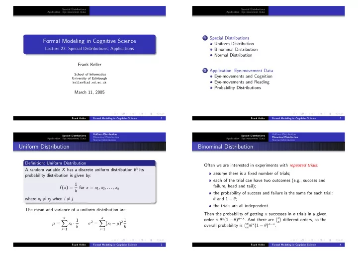
Special Distributions Special Distributions Application: Eye-movement Data Application: Eye-movement Data 1 Special Distributions Formal Modeling in Cognitive Science Uniform Distribution Lecture 27: Special Distributions; Applications Binominal Distribution Normal Distribution Frank Keller 2 Application: Eye-movement Data School of Informatics Eye-movements and Cognition University of Edinburgh Eye-movements and Reading keller@inf.ed.ac.uk Probability Distributions March 11, 2005 Frank Keller Formal Modeling in Cognitive Science 1 Frank Keller Formal Modeling in Cognitive Science 2 Uniform Distribution Uniform Distribution Special Distributions Special Distributions Binominal Distribution Binominal Distribution Application: Eye-movement Data Application: Eye-movement Data Normal Distribution Normal Distribution Uniform Distribution Binominal Distribution Definition: Uniform Distribution Often we are interested in experiments with repeated trials: A random variable X has a discrete uniform distribution iff its assume there is a fixed number of trials; probability distribution is given by: each of the trial can have two outcomes (e.g., success and f ( x ) = 1 failure, head and tail); k for x = x 1 , x 2 , . . . , x k the probability of success and failure is the same for each trial: where x i � = x j when i � = j . θ and 1 − θ ; the trials are all independent. The mean and variance of a uniform distribution are: Then the probability of getting x successes in n trials in a given k k � n order is θ x (1 − θ ) n − x . And there are � different orders, so the x i · 1 ( x i − µ ) 2 1 σ 2 = � � x µ = � n � θ x (1 − θ ) n − x . overall probability is k k x i =1 i =1 Frank Keller Formal Modeling in Cognitive Science 3 Frank Keller Formal Modeling in Cognitive Science 4

Uniform Distribution Uniform Distribution Special Distributions Special Distributions Binominal Distribution Binominal Distribution Application: Eye-movement Data Application: Eye-movement Data Normal Distribution Normal Distribution Binominal Distribution Binominal Distribution 1 Definition: Binomial Distribution 0.9 A random variable X has a binominal distribution iff its probability 0.8 distribution is given by: 0.7 � n � θ x (1 − θ ) n − x for x = 0 , 1 , 2 , . . . , n b(x; 12, 0.5) 0.6 b ( x ; n , θ ) = x 0.5 0.4 Example 0.3 The probability of getting five heads and seven tail in 12 flips of a 0.2 balanced coin is: 0.1 b (5; 12 , 1 � 12 � (1 2) 5 (1 − 1 2) 12 − 5 2) = 5 0 1 1 2 3 4 5 6 7 8 9 10 11 12 x Frank Keller Formal Modeling in Cognitive Science 5 Frank Keller Formal Modeling in Cognitive Science 6 Uniform Distribution Uniform Distribution Special Distributions Special Distributions Binominal Distribution Binominal Distribution Application: Eye-movement Data Application: Eye-movement Data Normal Distribution Normal Distribution Binominal Distribution Normal Distribution Definition: Normal Distribution If we invert successes and failures (or heads and tails), then the A random variable X has a normal distribution iff its probability probability stays the same. Therefore: density is given by: Theorem: Binomial Distribution 1 σ ) 2 for − ∞ < x < ∞ e − 1 2 ( x − µ n ( x ; µ, σ ) = √ b ( x ; n , θ ) = b ( n − x ; n , 1 − θ ) 2 π σ Two other important properties of the binomial distribution are: Normally distributed random variables are ubiquitous in Theorem: Binomial Distribution probability theory; The mean and the variance of the binomial distribution are: many measurements of physical, biological, or cognitive processes yield normally distributed data; σ 2 = n θ (1 − θ ) µ = n θ and such data can be modeled using a normal distributions (sometimes using mixtures of several normal distributions). Frank Keller Formal Modeling in Cognitive Science 7 Frank Keller Formal Modeling in Cognitive Science 8

Uniform Distribution Uniform Distribution Special Distributions Special Distributions Binominal Distribution Binominal Distribution Application: Eye-movement Data Application: Eye-movement Data Normal Distribution Normal Distribution Standard Normal Distribution Normal Distribution Definition: Standard Normal Distribution 0.4 The normal distribution with µ = 0 and σ = 1 is referred to as the standard normal distribution: 0.3 1 e − 1 2 x 2 √ n ( x ; 0 , 1) = 2 π 0.2 Theorem: Standard Normal Distribution If a random variable X has a normal distribution, then: 0.1 P ( | x − µ | < σ ) = 0 . 6826 P ( | x − µ | < 2 σ ) = 0 . 9544 0 -4 -2 0 2 4 This follows from Chebyshev’s Theorem (see previous lecture). x Frank Keller Formal Modeling in Cognitive Science 9 Frank Keller Formal Modeling in Cognitive Science 10 Uniform Distribution Eye-movements and Cognition Special Distributions Special Distributions Binominal Distribution Eye-movements and Reading Application: Eye-movement Data Application: Eye-movement Data Normal Distribution Probability Distributions Normal Distribution Eye-movements and Cognition Let’s apply what we’ve learned to some real data. Theorem: Z -Scores An eye-tracker makes it possible to record the eye-movements of If a random variable X has a normal distribution with the mean µ subjects while their are performing a cognitive task: and the standard deviation σ then: reading a text; Z = X − µ looking at a picture; σ using a computer screen and keyboard; has the standard normal distribution. driving a vehicle. This conversion is often used to make results obtained by different Mind’s Eye Hypothesis: where subjects are looking indicates what experiments comparable: convert the distributions to Z -scores. they are processing. How long they are looking at it indicates how much processing effort is needed. Frank Keller Formal Modeling in Cognitive Science 11 Frank Keller Formal Modeling in Cognitive Science 12

Eye-movements and Cognition Eye-movements and Cognition Special Distributions Special Distributions Eye-movements and Reading Eye-movements and Reading Application: Eye-movement Data Application: Eye-movement Data Probability Distributions Probability Distributions Eye-movements and Cognition Eye-movements and Reading Let’s look at subjects’ eye-movements while they read text. Frank Keller Formal Modeling in Cognitive Science 13 Frank Keller Formal Modeling in Cognitive Science 14 Eye-movements and Cognition Eye-movements and Cognition Special Distributions Special Distributions Eye-movements and Reading Eye-movements and Reading Application: Eye-movement Data Application: Eye-movement Data Probability Distributions Probability Distributions Eye-movements and Reading Eye-movements and Reading Frank Keller Formal Modeling in Cognitive Science 15 Frank Keller Formal Modeling in Cognitive Science 16

Eye-movements and Cognition Eye-movements and Cognition Special Distributions Special Distributions Eye-movements and Reading Eye-movements and Reading Application: Eye-movement Data Application: Eye-movement Data Probability Distributions Probability Distributions Eye-movements and Reading Probability Distributions Data: 23 subjects read a 2000 word text while their Eye-movements are recorded while subjects read texts; eye-movements were being recorded. very high spatial and temporal accuracy; To analyze the data, define two random variables: eye movements in reading are saccadic: a series of relatively X : time taken to read a word; stationary periods (fixations) between very fast movements (saccades); Y : number of regressions made while reading a word; average fixation time is about 250 ms; can be longer or Note that X is a continuous random variable, while Y is a discrete shorter, depending on ease or difficulty of processing; random variable. typically test a number of subjects, with a number of test Plot the distributions; compute their means and standard sentences, and statistical analysis done on results. deviations. Frank Keller Formal Modeling in Cognitive Science 17 Frank Keller Formal Modeling in Cognitive Science 18 Eye-movements and Cognition Eye-movements and Cognition Special Distributions Special Distributions Eye-movements and Reading Eye-movements and Reading Application: Eye-movement Data Application: Eye-movement Data Probability Distributions Probability Distributions Distribution: Reading Time Distribution: Number of Regressions 500 2000 450 1750 400 1500 350 1250 300 Frequency Frequency 1000 250 200 750 150 500 100 250 50 0 0 0 100 200 300 400 500 600 700 7 0 1 2 3 4 5 6 8 9 Fixation time [ms] Number of regressions µ = 269 . 58, σ = 132 . 88. Almost normal distribution. µ = 1 . 31, σ = 1 . 81. Almost a binominal distribution. Frank Keller Formal Modeling in Cognitive Science 19 Frank Keller Formal Modeling in Cognitive Science 20