Binomial and Normal Distributions Bernoulli Trials A Bernoulli - PowerPoint PPT Presentation
Binomial and Normal Distributions Bernoulli Trials A Bernoulli trial is a random experiment with 2 special properties: The result of a Bernoulli trial is binary. Examples: Heads vs. Tails, Healthy vs. Sick, etc. The probability
Binomial and Normal Distributions
Bernoulli Trials A Bernoulli trial is a random experiment with 2 special properties: The result of a Bernoulli trial is binary. ● Examples: Heads vs. Tails, Healthy vs. Sick, etc. ○ ● The probability of a “success” is some constant p . Example: the probability of heads when you flip a fair coin is always 50%. ○
Bernoulli Random Variable A Bernoulli random variable is a random variable such that: The range of possible values is binary. ● Examples: Heads vs. Tails, Healthy vs. Sick, etc. ○ ● The probability of a “success” is some constant p . Example: the probability of heads is p , and the probability of tails is 1-p . ○
Binomial Random Variable A binomial random variable describes the result of n Bernoulli trials: The range is the natural numbers, representing the number of successes. ● Examples: The number of heads, The number of healthy participants, etc. ○ ● The probability of a “success” is constant across all trials. Example: the probability of heads when you flip a fair coin is always 50%. ○ The trials are independent events; earlier trials do not influence later trials. ●
Examples of Binomial Random Variables The number of heads in 10 coin flips. ● ● The number of times you roll double sixes in 50 rolls of the dice. ● The number of people who quit smoking after treating 100 participants. The number of people who report that they prefer Clinton to Trump in a ● poll of 500 individuals (2016). ● What else?
The Binomial Distribution Here is the formula for the binomial distribution: ● X is the binomial random variable, k is the number of successes, n is the ● number of trials, and p is the probability of success. ● For example, let X be the total number of heads in 10 flips of a fair coin. This means k ranges from 0 to 10, n = 10, and p = 0.5.
Aside: Pascal’s Triangle (n choose k) = n ! / ( k ! ( n - k )!) ● Image source
Calculating Binomial Probabilities in R Assume a binomial random variable X with parameters n and p . ● The random variable can take on values of k ranging from 0 through n . ○ R can help us find Pr[ X = k ] for all values of k . ○ In R, we can use dbinom(k, n, p) to find Pr[ X = k ] ● Let’s say we flip a coin 10 times. What is the probability we see 3 heads? ○ dbinom(3, 10, 0.5) outputs 0.117 ○ In R, we can use pbinom(k, n, p) to find the Pr[ X ≤ k ] ● If we flip a coin 10 times, what is the probability we see 4 heads, or fewer? ○ dbinom(0, 10, 0.5) + dbinom(1, 10, 0.5) + dbinom(2, ○ 10, 0.5) + dbinom(3, 10, 0.5) outputs 0.172 pbinom(3, 10, 0.5) also outputs 0.172 ○
Expected Value and Variance Bernoulli random variable: The expected value of a Bernoulli random variable is p. ● E[ B ] = ( p )(1) + ( 1-p )(0) = p ○ ● The variance of a Bernoulli random variable is p(1-p) . E[( B - � ) 2 ] = ( p )( 1-p ) 2 + ( 1-p )( 0-p ) 2 = p(1-p) ○ E[B 2 ] - � 2 = ( p )(1 2 ) + ( 1-p )(0 2 ) - p 2 = p - p 2 = p(1-p) ○ Binomial random variable: The expected value of a binomial random variable is np . ● The variance of a binomial random variable is np(1-p) . ●
The Binomial Distribution The red distribution is binomial(10, 0.5)
The Binomial Distribution The blue distribution is binomial(10, 0.3) The red distribution is binomial(10, 0.5) The green distribution is binomial(10, 0.7)
Does this shape ring a bell?
The Normal Distribution ● A bell-shaped curve, whose shape depends on two things ○ Mean, Median, and Mode: the center of the curve ○ Standard deviation (or Variance): the spread (i.e., the height and width) of the curve Image source Image source
Central Limit Theorem
Central Limit Theorem Let’s consider rolling a die, say, 100 times, and computing the mean roll ● num_trials <- 100 sample_data <- sample(0:1, num_trials, replace = TRUE) mean(sample_data) And let’s repeat this process, first 10, then 100, and then 1000 times ●
Central Limit Theorem (cont’d) A histogram of sample means is called the sampling distribution. ● ● As we collect more and more sample means, the sampling distribution looks more and more like the normal distribution. This is true even though the distribution that we were sampling from was ● uniform (not normal). ● Amazing fact: this is true regardless of the underlying distribution.
Central Limit Theorem (cont’d) Regardless of the population distribution, in the limit (as the number of experiments grows to infinity), the sample mean is normally distributed around the population mean. But what is the standard deviation? The standard deviation of the sampling distribution is called standard error. ● Standard deviation measures variation within the population, meaning how much individual measurements differ from the mean. ● Standard error measures how much sample means differ from the population mean.
Are data normally normally distributed? Students in a statistics class at Simon Fraser University. Image source
Recommend
More recommend
Explore More Topics
Stay informed with curated content and fresh updates.
