k-Maximum Likelihood Estimator for mixtures of generalized Gaussians - PowerPoint PPT Presentation
Motivation and background k -Maximum Likelihood estimator Mixtures of generalized Gaussian distribution k-Maximum Likelihood Estimator for mixtures of generalized Gaussians ICPR 2012, Tokyo, Japan Olivier Schwander Aurlien Schutz Yannick
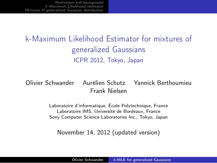
Motivation and background k -Maximum Likelihood estimator Mixtures of generalized Gaussian distribution k-Maximum Likelihood Estimator for mixtures of generalized Gaussians ICPR 2012, Tokyo, Japan Olivier Schwander Aurélien Schutz Yannick Berthoumieu Frank Nielsen Laboratoire d’informatique, École Polytechnique, France Laboratoire IMS, Université de Bordeaux, France Sony Computer Science Laboratories Inc., Tokyo, Japan November 14, 2012 (updated version) Olivier Schwander k-MLE for generalized Gaussians
Motivation and background k -Maximum Likelihood estimator Mixtures of generalized Gaussian distribution Outline Motivation and background Target applications Generalized Gaussian Exponential families k -Maximum Likelihood estimator Complete log-likelihood Algorithm Key points Mixtures of generalized Gaussian distribution Direct applications of k -MLE Rewriting complete log-likelihood Experiments Olivier Schwander k-MLE for generalized Gaussians
Motivation and background Target applications k -Maximum Likelihood estimator Generalized Gaussian Mixtures of generalized Gaussian distribution Exponential families Textures Brodatz Description ◮ Wavelet transform Tasks ◮ Classification ◮ Retrieval Olivier Schwander k-MLE for generalized Gaussians
Motivation and background Target applications k -Maximum Likelihood estimator Generalized Gaussian Mixtures of generalized Gaussian distribution Exponential families Popular models Modeling wavelet coefficient distribution ◮ generalized Gaussian distribution (Do 2002, Mallat 1996) ◮ mixture of generalized Gaussian distributions (Allili 2012) Olivier Schwander k-MLE for generalized Gaussians
Motivation and background Target applications k -Maximum Likelihood estimator Generalized Gaussian Mixtures of generalized Gaussian distribution Exponential families Generalized Gaussian Definition � � −| x − µ | β β f ( x ; µ, α, β ) = 2 α Γ( 1 /β ) exp α ◮ µ : mean (real number) ◮ α : scale (positive real number) ◮ β : shape (positive real number) Multivariate version: a product of one dimensional laws Olivier Schwander k-MLE for generalized Gaussians
Motivation and background Target applications k -Maximum Likelihood estimator Generalized Gaussian Mixtures of generalized Gaussian distribution Exponential families Properties and examples Contains ◮ Gaussian β = 2 ◮ Laplace β = 1 0 . 20 β = 0.5 β = 1.0 ◮ Uniform β → ∞ β = 2.0 β = 10.0 0 . 15 Maximum likelihood estimator 0 . 10 ◮ Iterative procedure (Newton-Raphson) 0 . 05 Exponential family 0 . 00 − 10 − 5 0 5 10 ◮ For a fixed β Olivier Schwander k-MLE for generalized Gaussians
Motivation and background Target applications k -Maximum Likelihood estimator Generalized Gaussian Mixtures of generalized Gaussian distribution Exponential families Exponential families Definition p ( x ; λ ) = p F ( x ; θ ) = exp ( � t ( x ) | θ � − F ( θ ) + k ( x )) ◮ λ source parameter Generalized Gaussian ◮ t ( x ) sufficient statistic Fixed µ and β ◮ θ natural parameter ◮ t ( x ) = −| x − µ | β ◮ F ( θ ) log-normalizer ◮ θ = α − β ◮ k ( x ) carrier measure ◮ F ( θ ) = � � β F is a stricly convex and − β log ( θ ) + log 2 Γ( 1 /β ) differentiable function ◮ k ( x ) = 0 �·|·� is a scalar product Olivier Schwander k-MLE for generalized Gaussians
Motivation and background Target applications k -Maximum Likelihood estimator Generalized Gaussian Mixtures of generalized Gaussian distribution Exponential families A large class of distributions Gaussian or normal (generic, isotropic Gaussian, diagonal Gaussian, rectified Gaussian or Wald distributions, log-normal), Poisson, Bernoulli, binomial, multinomial (trinomial, Hardy-Weinberg distribution), Laplacian, Gamma (including the chi-squared), Beta, exponential, Wishart, Dirichlet, Rayleigh, probability simplex, negative binomial distribution, Weibull, Fisher-von Mises, Pareto distributions, skew logistic, hyperbolic secant, negative binomial, etc. With a large set of tools ◮ Bregman Soft Clustering (EM like algorithm) ◮ Bregman Hard Clustering ( k -means like algorithm) ◮ Kullback-Leibler divergence (through Bregman divergence) Strong links with the Bregman divergences (Banerjee 2005) Olivier Schwander k-MLE for generalized Gaussians
Motivation and background Target applications k -Maximum Likelihood estimator Generalized Gaussian Mixtures of generalized Gaussian distribution Exponential families Bregman divergence Definition and properties ◮ B F ( p , q ) = F ( p ) − F ( q ) + � p − q |∇ F ( q ) � ◮ F is a stricly convex and differentiable function ◮ Centroids known in closed-form Legendre duality ◮ F ⋆ ( η ) = sup θ {� θ, η � − F ( θ ) } ◮ η = ∇ F ( θ ) , θ = ∇ F ⋆ ( η ) Bijection with exponential families log p F ( x | θ ) = − B F ∗ ( t ( x ) : η ) + F ∗ ( t ( x )) + k ( x ) Olivier Schwander k-MLE for generalized Gaussians
Motivation and background Complete log-likelihood k -Maximum Likelihood estimator Algorithm Mixtures of generalized Gaussian distribution Key points Usual setup: expectation-maximization Joint probability with missing component labels ◮ Observations from a finite mixture � p ( x 1 , z 1 , . . . , x n , z n ) = p ( z i | ω ) p ( x i | z i , θ ) i ◮ Marginalization � � p ( x 1 , . . . , x n | ω, θ ) = p ( z i = j | ω ) p ( x i | z i = j , θ ) i j EM maximizes l = 1 n log p ( x 1 , . . . , z n ) = 1 � � ¯ log p ( z i = j | ω ) p ( x i | z i = j , θ ) n i j Olivier Schwander k-MLE for generalized Gaussians
Motivation and background Complete log-likelihood k -Maximum Likelihood estimator Algorithm Mixtures of generalized Gaussian distribution Key points Complete log-likelihood Complete average log-likelihood l ′ = 1 n log p ( x 1 , z 1 , . . . , x n , z n ) = 1 � ( ω j p ( x i , θ j )) δ ( z i ) � � � ¯ log n i j = 1 � � δ ( z i ) ( log p ( x i , θ j ) + log ω j ) n i j But p is an exponential family log p ( x i , θ j ) = log p F ( x i , θ j ) = − B F ∗ ( t ( x ) , η j ) + F ⋆ ( t ( x )) + k ( x ) � �� � does not depend on θ Olivier Schwander k-MLE for generalized Gaussians
Motivation and background Complete log-likelihood k -Maximum Likelihood estimator Algorithm Mixtures of generalized Gaussian distribution Key points With fixed weights Equivalent problem ◮ Minimizing l ′ = 1 � � − ¯ δ ( z i ) ( B F ∗ ( t ( x ) , η j ) − log ω j ) n i j = 1 � min ( B F ∗ ( t ( x ) , η j ) − log ω j ) n j i Bregman k -means with B F ⋆ − log ω j for divergence Olivier Schwander k-MLE for generalized Gaussians
Motivation and background Complete log-likelihood k -Maximum Likelihood estimator Algorithm Mixtures of generalized Gaussian distribution Key points k -Maximum Likelihood estimator Nielsen 2012 Initialization 1. Initialization (random or k -MLE++) 2. Assignment z i = arg min B F ⋆ − log ω j Assignment Until convergence (gives a partition in cluster C j ) 3. Update of the η j parameters Until convergence � 1 x ∈ C i t ( x ) (Bregman η j = | C j | Update centroid) parameters 4. Goto step 2 until local convergence 5. Update of the weights ω j = | C j | n Update 6. Goto step 2 until local convergence weights Olivier Schwander k-MLE for generalized Gaussians
Motivation and background Complete log-likelihood k -Maximum Likelihood estimator Algorithm Mixtures of generalized Gaussian distribution Key points Key points k -MLE ◮ optimizes the complete log-likelihood ◮ is faster than EM ◮ converges finitely to a local maximum Limitations ◮ All the components must belong to the same family ◮ F ⋆ may be difficult to compute (without closed form) What if each component belongs to a different EF ? Olivier Schwander k-MLE for generalized Gaussians
Motivation and background Direct applications of k -MLE k -Maximum Likelihood estimator Rewriting complete log-likelihood Mixtures of generalized Gaussian distribution Experiments Direct applications of k -MLE or of EM (Bregman Soft Clustering) A mixture model ◮ with all components in same the mixture model ◮ generalized Gaussian sharing the same µ : same mean ◮ generalized Gaussian sharing the same β : same shape ◮ one degree of freedom: α (scale) May be useful ◮ See mixtures of Laplace distributions ( β = 1) Not enough for texture description Olivier Schwander k-MLE for generalized Gaussians
Motivation and background Direct applications of k -MLE k -Maximum Likelihood estimator Rewriting complete log-likelihood Mixtures of generalized Gaussian distribution Experiments Complete log-likelihood revisited Complete average log-likelihood l ′ = 1 n log p ( x 1 , z 1 , . . . , x n , z n ) = 1 � � ¯ δ ( z i ) ( log p ( x i , θ j ) + log ω j ) n i j Each component is an exponential family n k l ′ = 1 � � � � ¯ − B F j ∗ ( t ( x i ) : η j ) + F j ∗ ( t ( x i )) + k j ( x i ) + log ω j δ j ( z i ) n i = 1 j = 1 � �� � − U j ( x i ,η j ) Olivier Schwander k-MLE for generalized Gaussians
Recommend
More recommend
Explore More Topics
Stay informed with curated content and fresh updates.
